Day 2 - Module 08: Count normalizations and DESeq2 model fitting

Objectives:

• Discuss count normalizations
• Execute model fitting for differential expression comparisons

1 Differential Expression Workflow

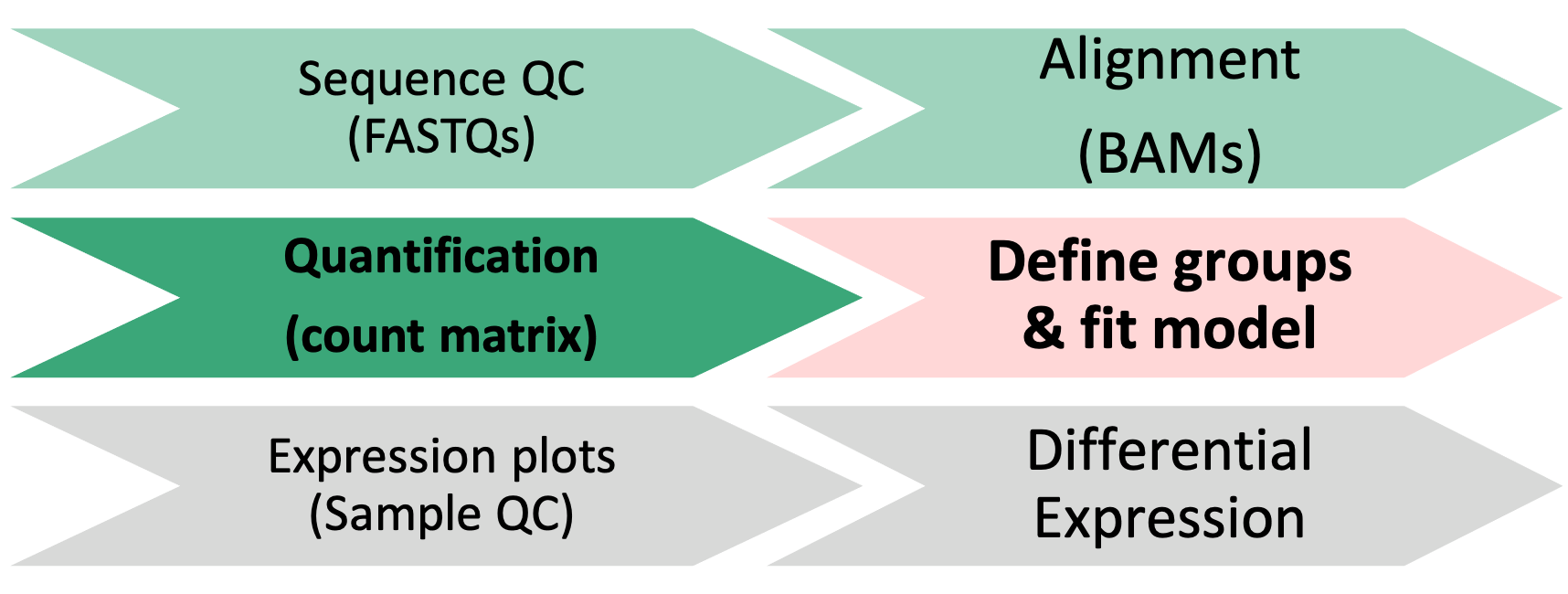
Here we will proceed with count normalizations and fit our DESeq2 model.

---

2 Count normalizations

Since counts of mapped reads for each gene is proportional to the expression of RNA in addition to many “uninteresting” other factors, normalization is the process of scaling raw count values to account for the “uninteresting” factors and ensure expression levels are more comparable.

2.1 Normalization goals

Two common factors that need to be accounted for during normalization are sequencing depth and gene length. Common normalization approaches (such as FPKM, RPKM, CPM, TPM, etc.) account for one or both of these factors.

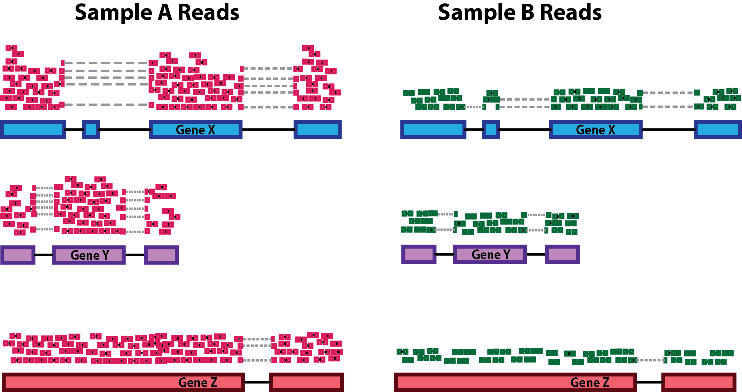
• Sequencing depth normalization is necessary to account for the proportion of reads per gene expected for more deeply sequenced samples (like in pink below) versus a less deeply sequenced sample (like in green below).

Note that each pink or green rectangle represents an aligned read, with reads spanning an intron connected by a dashed line. Figure from HBC training materials

• Gene length normalization may also be necessary if comparing between different genes, since genes of different lengths have different probabilities of generating fragments that end up in the library.

Note: The above figure was originally from a HBC tutorial that also includes a detailed comparison of different normalization (CPM, TPM, FPKM) approaches and their best uses.

Check-in: Questions about normalizations?

2.2 DESeq2 normalizations

DESeq2 has an internal normalization process that accounts for RNA composition. A few highly differentially expressed genes, differences in the number of genes expressed between samples, or contamination are not accounted for by depth or gene length normalization methods. Accounting for RNA composition is particularly important for differential expression analyses, regardless of the tool used.

For data exploration and visualizations, it is helpful to generate an object of independently normalized counts. We will use the rlog transformation from DESeq2 that accounts for sequencing depth for each sample and RNA composition for the downstream quality control visualizations.

The rlog transformation produces log2 scale data that has also been normalized to overall library size as well as variance across genes at different mean expression levels. For larger numbers of samples, there is an alternative transformation method, vst that can be used instead for count normalizations.

The command to generate the normalized count object has a few parts, including dds as an input and providing a value to the option blind.

rld <- rlog(dds, blind = TRUE)

*Note: We might see a message that our data did not fit the default ‘parametric’ dispersion model so a local regression was substituted. If we had more time, we might look at a dispersion plot with the plotDispEsts(dds) function, but as this bioconductor thread discusses, other visualizations of our data might be more helpful and/or easier to interpret.

Next, we’ll look at the results of the transformation.

head(assay(rld), 2)

##                    Sample_116498 Sample_116499 Sample_116500 Sample_116501 Sample_116502
## ENSMUSG00000000001     12.635215     12.609457      12.76686     12.616921     12.705707
## ENSMUSG00000000028      8.096766      8.350835       8.17923      8.391328      8.616073
##                    Sample_116503 Sample_116504 Sample_116505 Sample_116506 Sample_116507
## ENSMUSG00000000001     12.661095      12.54194      12.52138      12.49388      12.71019
## ENSMUSG00000000028      8.653318      10.71402      10.77955      10.88032      11.01995
##                    Sample_116508 Sample_116509
## ENSMUSG00000000001      12.52632      12.48844
## ENSMUSG00000000028      10.93564      10.96100

Looking at the rld values, we can see that they are now in log scale. Since we set blind=TRUE, the transformation is blind to the sample information we specified in the design formula. The normalized counts are helpful for visualization methods during expression-level quality assessment but aren’t used in the model fitting.

3 DESeq2 Model Fitting

Next, we’ll fit our standard model using the DESeq function and take a look at the objects we generate.

dds <- DESeq(dds)

This command applies the model to our data, using the sample information supplied when generating the dds object so it takes some time to run.

resultsNames(dds)

## [1] "Intercept"                    "Gtype.Tx_ko.Tx_vs_wt.Tx"      "Gtype.Tx_ko.control_vs_wt.Tx"
## [4] "Gtype.Tx_wt.control_vs_wt.Tx"

The results include three pairwise comparisons to the specified control as default, but other information is now stored in the dds object so we can generate additional pairwise comparisons of interest.

head(dds)

Checkpoint: If you see the same results when you execute resultsNames(dds), please indicate with the green ‘yes’ button. Otherwise, please use the red ‘x’ button to get help before the break

3.0.0.1 [Optional Exercise]

If you executed the commands in the option exercise from Module 07, you can fit a seperate DESeq2 model for the patient sample example, which included a covariate in our model.

Click for fitting a model that includes a covariate

dds_patient <- DESeq(dds_patient)

resultsNames(dds_patient)

If you run through the optional exercises, you can explore the impact of adding a covariate by substituting dds_patient for dds and re-running those commands since both DESeq2 objects have their data organized in the same way.

4 Summary

In this section, we:

• Learned about count normalizations and uses
  
• Generated a normalized count table
  
• Fit two DESeq2 models for our data
  
• Saw the impact of including a covariate in our model

---

5 Sources

5.1 Training resources used to develop materials

• HBC DGE setup: https://hbctraining.github.io/DGE_workshop/lessons/01_DGE_setup_and_overview.html
• HBC Count Normalization: https://hbctraining.github.io/DGE_workshop/lessons/02_DGE_count_normalization.html
• DESeq2 standard vignette: http://bioconductor.org/packages/devel/bioc/vignettes/DESeq2/inst/doc/DESeq2.html
• DESeq2 beginners vignette: https://bioc.ism.ac.jp/packages/2.14/bioc/vignettes/DESeq2/inst/doc/beginner.pdf
• Bioconductor RNA-seq Workflows: https://www.bioconductor.org/help/course-materials/2015/LearnBioconductorFeb2015/B02.1_RNASeq.html

These materials have been adapted and extended from materials listed above. These are open access materials distributed under the terms of the Creative Commons Attribution license (CC BY 4.0), which permits unrestricted use, distribution, and reproduction in any medium, provided the original author and source are credited.