R Bonus Content

Objectives

• Additional visualizations for gene/sample level QC assessment

Count boxplots

To evaluate the difference between the count distributions before and after normalization, let’s extract the raw counts and the rlog normalized counts, and coerce them to tibbles.

raw_counts = as_tibble(counts(dds), rownames = 'id')
norm_counts = as_tibble(assay(rld), rownames = 'id')

raw_counts

# A tibble: 55,492 × 7
   id                 sample_A sample_B sample_C sample_D sample_E sample_F
   <chr>                 <int>    <int>    <int>    <int>    <int>    <int>
 1 ENSMUSG00000000001     1041      905     1296     3481     1283     1921
 2 ENSMUSG00000000003        0        0        0        0        0        0
 3 ENSMUSG00000000028     1043     1232     1664     2690     1825     2720
 4 ENSMUSG00000000031     1819      914     1618     8618     1350     1222
 5 ENSMUSG00000000037       19       11       18       48       37       29
 6 ENSMUSG00000000049       18        1        4       24        1        1
 7 ENSMUSG00000000056    14972    14768    21026    22962    22263    23622
 8 ENSMUSG00000000058        1        0        0        0        0        0
 9 ENSMUSG00000000078      888      607      911     1689      738     1180
10 ENSMUSG00000000085      402      483      744      898      811     1261
# … with 55,482 more rows

norm_counts

# A tibble: 16,249 × 7
   id                 sample_A sample_B sample_C sample_D sample_E sample_F
   <chr>                 <dbl>    <dbl>    <dbl>    <dbl>    <dbl>    <dbl>
 1 ENSMUSG00000000001    10.5     10.4     10.4     10.8     10.4     10.6 
 2 ENSMUSG00000000028    10.6     10.7     10.7     10.7     10.8     11.0 
 3 ENSMUSG00000000031    11.2     10.5     10.7     11.9     10.6     10.3 
 4 ENSMUSG00000000037     4.64     4.56     4.58     4.66     4.72     4.62
 5 ENSMUSG00000000049     3.02     2.82     2.84     2.94     2.81     2.81
 6 ENSMUSG00000000056    14.3     14.3     14.3     13.9     14.4     14.2 
 7 ENSMUSG00000000078    10.1      9.77     9.86     9.93     9.68     9.90
 8 ENSMUSG00000000085     9.28     9.41     9.53     9.23     9.60     9.80
 9 ENSMUSG00000000088    10.4     10.6     10.7     10.5     10.5     10.2 
10 ENSMUSG00000000093     3.88     3.89     3.93     3.91     3.94     3.99
# … with 16,239 more rows

Next, this is the perfect opportunity to use tidyr::pivot_longer() because we want to use ggplot() for the bar plots, but the data is currently in the wide form, not the tidy form!

tidy_raw = tidyr::pivot_longer(raw_counts, -id, names_to = 'sample', values_to = 'counts')
tidy_norm = tidyr::pivot_longer(norm_counts, -id, names_to = 'sample', values_to = 'counts')

We should also join in the sample metadata so that we can color on the sample groups.

samplesheet_tbl = as_tibble(colData(dds), rownames = 'sample')

tidy_raw = tidy_raw %>% left_join(samplesheet_tbl, by = 'sample')
tidy_norm = tidy_norm %>% left_join(samplesheet_tbl, by = 'sample')

raw_boxplot = ggplot(tidy_raw, aes(x = sample, y = log2(counts), fill = condition)) +
    geom_boxplot(notch = TRUE) +
    labs(
        title = 'Raw Counts',
        x = 'Sample',
        y = 'log2 Counts') +
    theme_bw() + theme(axis.text.x = element_text(angle = 90))
raw_boxplot

Warning: Removed 226538 rows containing non-finite values (`stat_boxplot()`).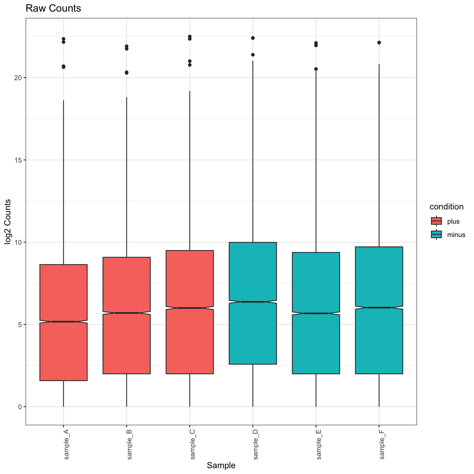

Question

Why did we get that warning about non-finite values?

norm_boxplot = ggplot(tidy_norm, aes(x = sample, y = counts, fill = condition)) +
    geom_boxplot(notch = TRUE) +
    labs(
        title = 'rlog Normalized Counts',
        x = 'Sample',
        y = 'rlog Counts') +
    theme_bw() + theme(axis.text.x = element_text(angle = 90))
norm_boxplot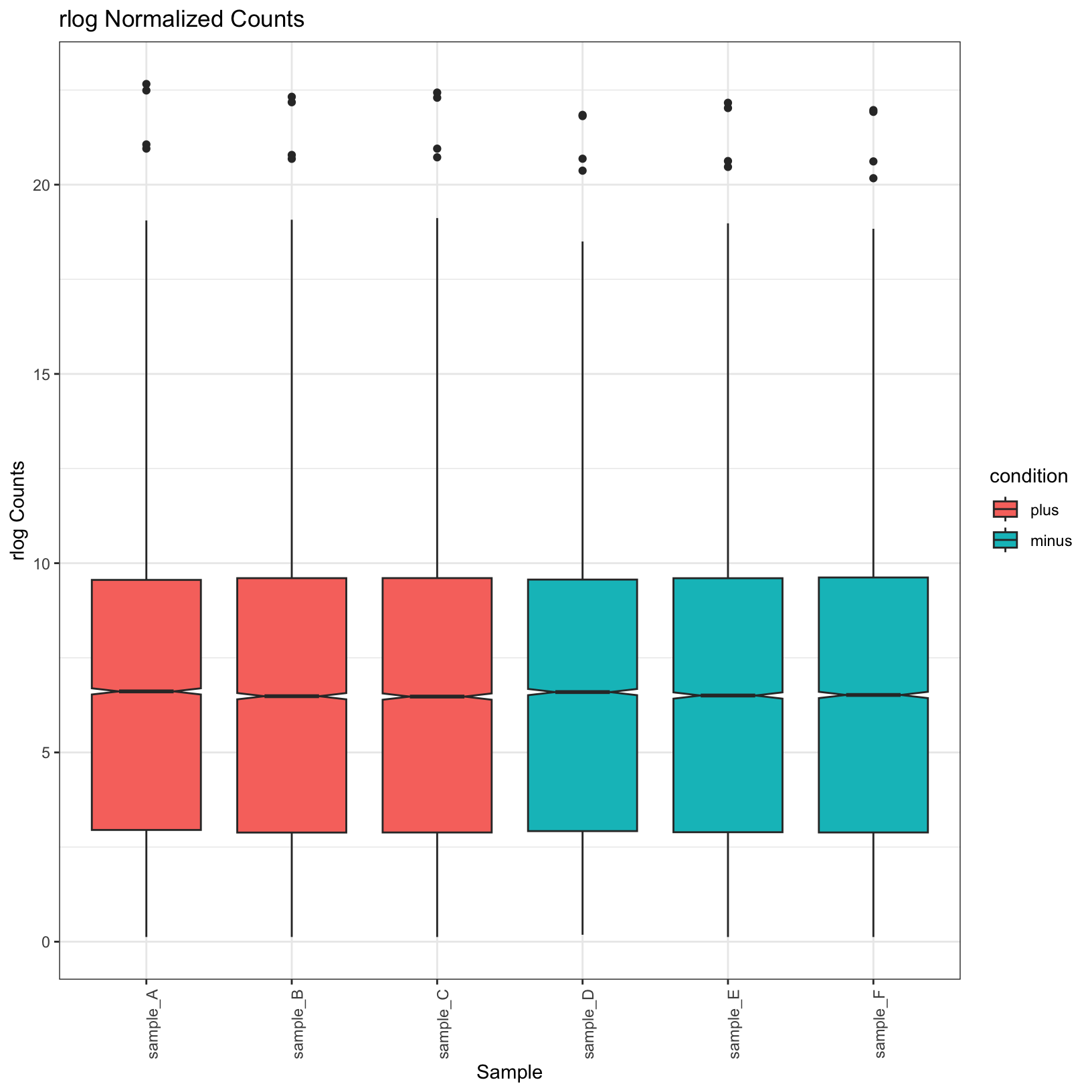

Observe that the normalized plots truly do appear normalized; their means are more uniform. Let’s go ahead and save these plots in our outputs/figures folder.

ggsave(filename = 'outputs/figures/Boxplot_raw_condition.pdf', plot = raw_boxplot, height = 6, width = 6)
ggsave(filename = 'outputs/figures/Boxplot_rlog_condition.pdf', plot = norm_boxplot, height = 6, width = 6)

Heatmaps

Let’s create a heatmap based on the distance between pair-wise sample expression profiles. This is another vantage point of how similar and dissimilar the samples are from one another. To get started, we actually want a plain matrix, with out a column for the gene IDs, as we did for the boxplot.

norm_mat = assay(rld)
head(norm_mat)

                    sample_A  sample_B  sample_C  sample_D  sample_E  sample_F
ENSMUSG00000000001 10.514813 10.366709 10.419463 10.840373 10.410449 10.578771
ENSMUSG00000000028 10.604461 10.734506 10.735026 10.682714 10.820938 10.990999
ENSMUSG00000000031 11.160276 10.498747 10.742763 11.861617 10.578156 10.298022
ENSMUSG00000000037  4.642433  4.555500  4.578934  4.656950  4.719012  4.620204
ENSMUSG00000000049  3.017478  2.820198  2.843894  2.936455  2.814833  2.811619
ENSMUSG00000000056 14.321672 14.284652 14.337197 13.904238 14.393912 14.235971

Next, we’ll use the dist() function on the transpose of norm_mat to compute the distance. We will use the default Euclidean distance.

dist_mat = dist(t(norm_mat), upper = TRUE)

Next, we’ll plot a very simple pheatmap() using this matrix. But let’s check the class of dist_mat first, because the input to pheatmap() needs to be a matrix.

class(dist_mat)

[1] "dist"

# Have to coerce it
dist_mat = as.matrix(dist_mat)

dist_heatmap = pheatmap(
    mat = dist_mat,
    cluster_rows = TRUE,
    cluster_cols = TRUE,
    show_rownames = TRUE,
    show_colnames = TRUE
)
dist_heatmap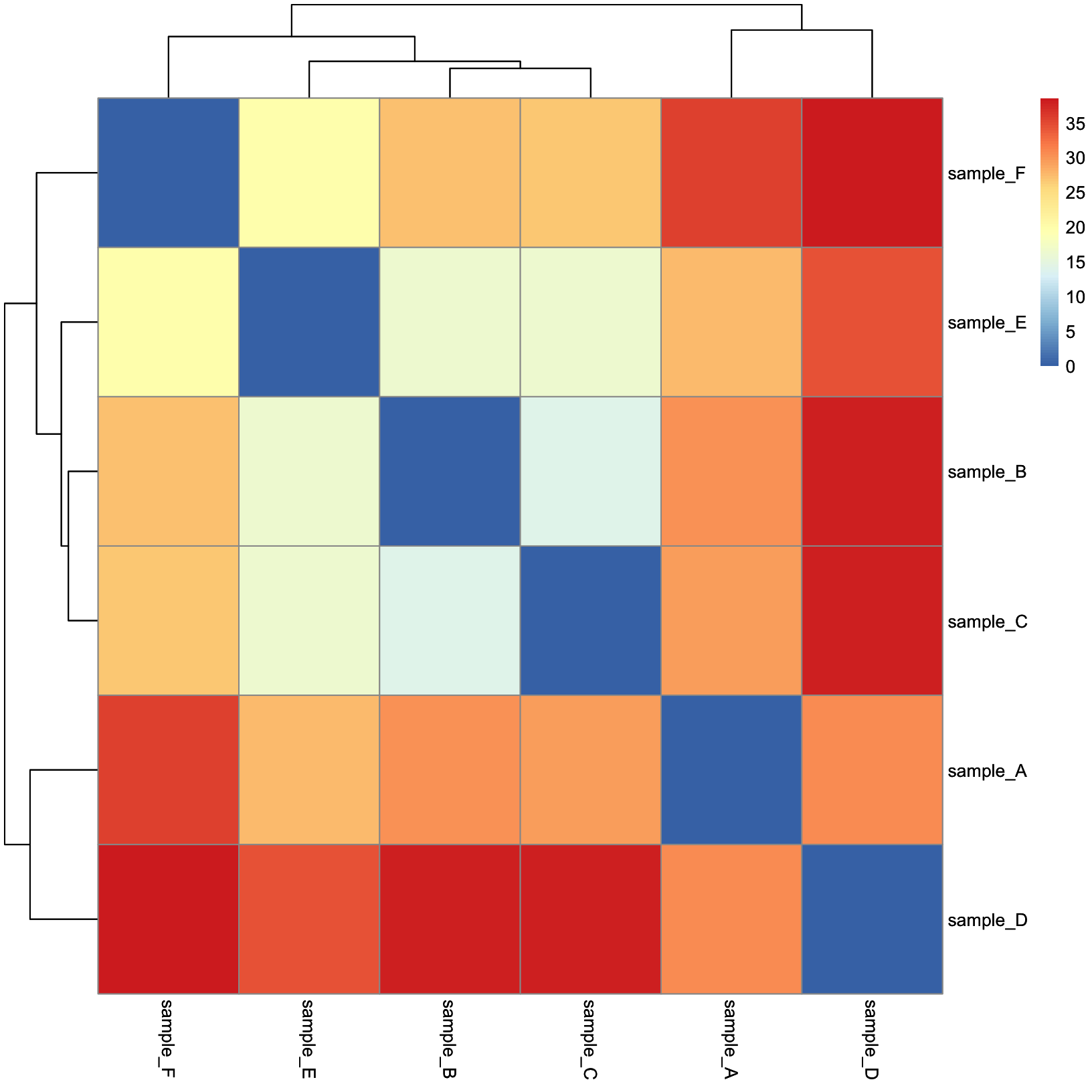

This is nice, but there are a few tweaks we might consider:

1. The color scale used by default is divergent, but our distances are values in [0, Inf), so a linear color scale would be more appropriate here.
2. We might like for the sample metadata to be included so that we can easily tell if the samples cluster by their condition.

To accomplish the first change, we’ll use the colorRampPalette() function from the RColorBrewer package. This is the package to use for creating color scales of all varieties. We highly recommend exploring the package website and documentation.

colors = colorRampPalette(brewer.pal(9, 'Blues'))(50)

Now let’s use that in the pheatmap() call using the color parameter:

dist_heatmap = pheatmap(
    mat = dist_mat,
    color = colors,
    cluster_rows = TRUE,
    cluster_cols = TRUE,
    show_rownames = TRUE,
    show_colnames = TRUE
)
dist_heatmap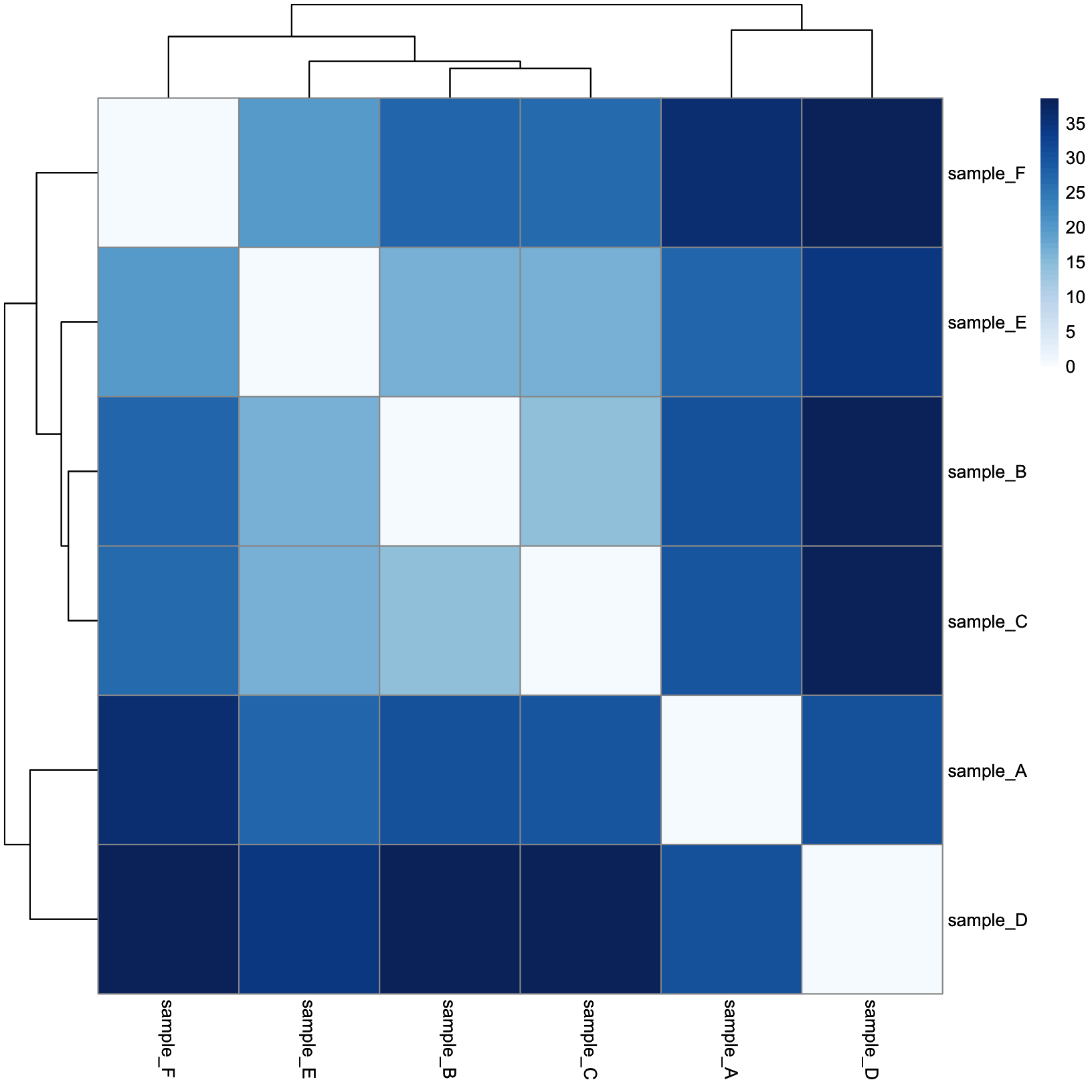

This is a lot more reasonable. More distant samples are a deeper blue, while more similar samples are closer to white. Next, let’s add some annotation data.

annotation_tbl = samplesheet_tbl %>%
    dplyr::select(sample, condition) %>%
    tibble::column_to_rownames(var = 'sample')

dist_heatmap = pheatmap(
    mat = dist_mat,
    color = colors,
    cluster_rows = TRUE,
    cluster_cols = TRUE,
    show_rownames = TRUE,
    show_colnames = TRUE,
    annotation_col = annotation_tbl
)
dist_heatmap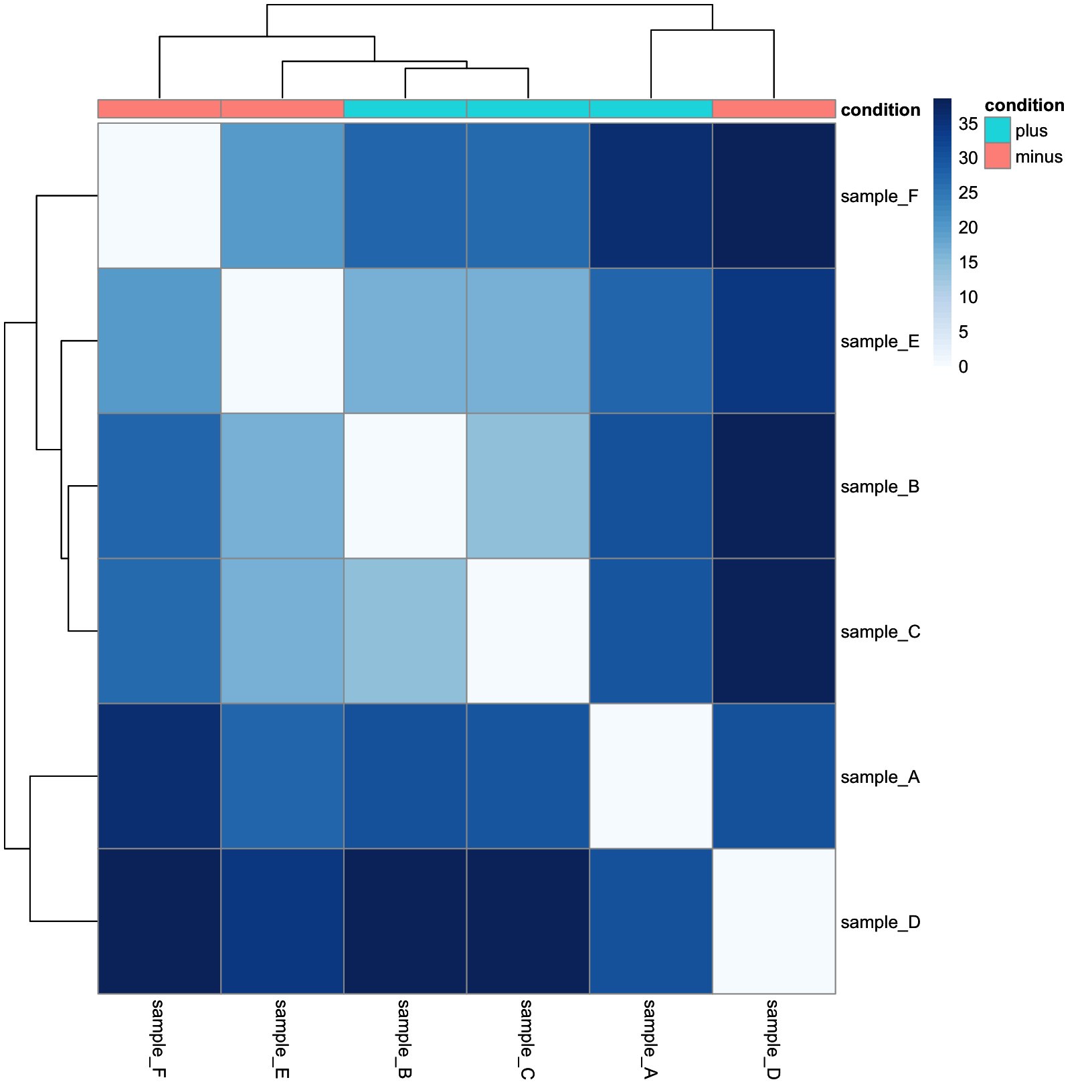

And now we have our conditions as a colored annotation bar along the columns.

Sources

• HBC QC tutorial: https://hbctraining.github.io/DGE_workshop/lessons/03_DGE_QC_analysis.html
• Detailed Heatmap tutorial from Galaxy: https://training.galaxyproject.org/training-material/topics/transcriptomics/tutorials/rna-seq-viz-with-heatmap2/tutorial.html

---

Session Info

sessionInfo()

R version 4.2.0 (2022-04-22)
Platform: x86_64-apple-darwin17.0 (64-bit)
Running under: macOS 13.2.1

Matrix products: default
LAPACK: /Library/Frameworks/R.framework/Versions/4.2/Resources/lib/libRlapack.dylib

locale:
[1] en_US.UTF-8/en_US.UTF-8/en_US.UTF-8/C/en_US.UTF-8/en_US.UTF-8

attached base packages:
[1] stats4    stats     graphics  grDevices utils     datasets  methods   base     

other attached packages:
 [1] biomaRt_2.52.0              knitr_1.41                  rmarkdown_2.18             
 [4] data.table_1.14.6           RColorBrewer_1.1-3          pheatmap_1.0.12            
 [7] ggrepel_0.9.2               DESeq2_1.36.0               SummarizedExperiment_1.26.1
[10] Biobase_2.56.0              MatrixGenerics_1.8.1        matrixStats_0.63.0         
[13] GenomicRanges_1.48.0        GenomeInfoDb_1.32.4         IRanges_2.30.1             
[16] S4Vectors_0.34.0            BiocGenerics_0.42.0         forcats_0.5.2              
[19] stringr_1.5.0               dplyr_1.0.10                purrr_0.3.5                
[22] readr_2.1.3                 tidyr_1.2.1                 tibble_3.1.8               
[25] ggplot2_3.4.0               tidyverse_1.3.2            

loaded via a namespace (and not attached):
 [1] googledrive_2.0.0      colorspace_2.0-3       ellipsis_0.3.2         XVector_0.36.0        
 [5] fs_1.5.2               rstudioapi_0.14        farver_2.1.1           bit64_4.0.5           
 [9] AnnotationDbi_1.58.0   fansi_1.0.3            lubridate_1.9.0        xml2_1.3.3            
[13] codetools_0.2-18       splines_4.2.0          cachem_1.0.6           geneplotter_1.74.0    
[17] jsonlite_1.8.3         broom_1.0.1            annotate_1.74.0        dbplyr_2.2.1          
[21] png_0.1-8              compiler_4.2.0         httr_1.4.4             backports_1.4.1       
[25] assertthat_0.2.1       Matrix_1.5-3           fastmap_1.1.0          gargle_1.2.1          
[29] cli_3.4.1              prettyunits_1.1.1      htmltools_0.5.3        tools_4.2.0           
[33] gtable_0.3.1           glue_1.6.2             GenomeInfoDbData_1.2.8 rappdirs_0.3.3        
[37] Rcpp_1.0.9             cellranger_1.1.0       jquerylib_0.1.4        vctrs_0.5.1           
[41] Biostrings_2.64.1      xfun_0.35              rvest_1.0.3            timechange_0.1.1      
[45] lifecycle_1.0.3        XML_3.99-0.13          googlesheets4_1.0.1    zlibbioc_1.42.0       
[49] scales_1.2.1           vroom_1.6.0            hms_1.1.2              parallel_4.2.0        
[53] curl_4.3.3             yaml_2.3.6             memoise_2.0.1          sass_0.4.4            
[57] stringi_1.7.8          RSQLite_2.2.19         highr_0.9              genefilter_1.78.0     
[61] filelock_1.0.2         BiocParallel_1.30.4    rlang_1.0.6            pkgconfig_2.0.3       
[65] bitops_1.0-7           evaluate_0.18          lattice_0.20-45        labeling_0.4.2        
[69] bit_4.0.5              tidyselect_1.2.0       magrittr_2.0.3         R6_2.5.1              
[73] generics_0.1.3         DelayedArray_0.22.0    DBI_1.1.3              pillar_1.8.1          
[77] haven_2.5.1            withr_2.5.0            survival_3.4-0         KEGGREST_1.36.3       
[81] RCurl_1.98-1.9         modelr_0.1.10          crayon_1.5.2           utf8_1.2.2            
[85] BiocFileCache_2.4.0    tzdb_0.3.0             progress_1.2.2         locfit_1.5-9.6        
[89] grid_4.2.0             readxl_1.4.1           blob_1.2.3             reprex_2.0.2          
[93] digest_0.6.30          xtable_1.8-4           munsell_0.5.0          bslib_0.4.1           

---

These materials have been adapted and extended from materials listed above. These are open access materials distributed under the terms of the Creative Commons Attribution license (CC BY 4.0), which permits unrestricted use, distribution, and reproduction in any medium, provided the original author and source are credited.