Objectives

Introduce R and RStudio.
Learn how to read in a csv file.
Discuss object naming conventions and types.
Discuss functions and parameters.
Learn how to get help with functions.
Get comfortable with errors and asking for help.

The gapminder dataset

We will be using a dataset from gapminder which contains life expectancy, GDP, and population for countries around the world from 1952 to 2007. It is sufficiently rich to allow us to explore data manipulation and visualization in R. We’ll begin with data just from 1997, and will expand to the full 1952 - 2007 dataset towards the end. The following is a preview of the data we’ll be working with:

gapminder preview

Create a project

We will create an RStudio Project to easily keep track of our working directory. See the Projects section of R for Data Science for a more in-depth description of what a project is and how it’s helpful.

To create a Project, click File then New Project…. In the New Project Wizard window that opens, select Existing Directory, then Browse…. In the Choose Directory window, select the IRR folder by clicking it once, and then click the Choose button. Finally, click Create Project.

Once we do this, RStudio will restart and the Files pane (lower right) should put us in the ~/IRR folder where there is an inputs/ folder and an IRR.Rproj file.

Checkpoint

The RStudio interface

RStudio is an integrated development environment where you can write, execute, and see the results of your code. The interface is arranged in different panes:

The Console pane along the left where you can enter commands and execute them.
The Environment pane in the upper right shows any variables you have created, along with their values.
The pane in the lower right has a few functions:
- The Files tab let’s you navigate the file system.
- The Plots tab displays any plots from code run in the Console.
- The Help tab displays the documentation of functions.

Commands in the Console

Working directly in the console is working directly with R. Commands can be entered and run with the Enter key:

> 2+2
[1] 4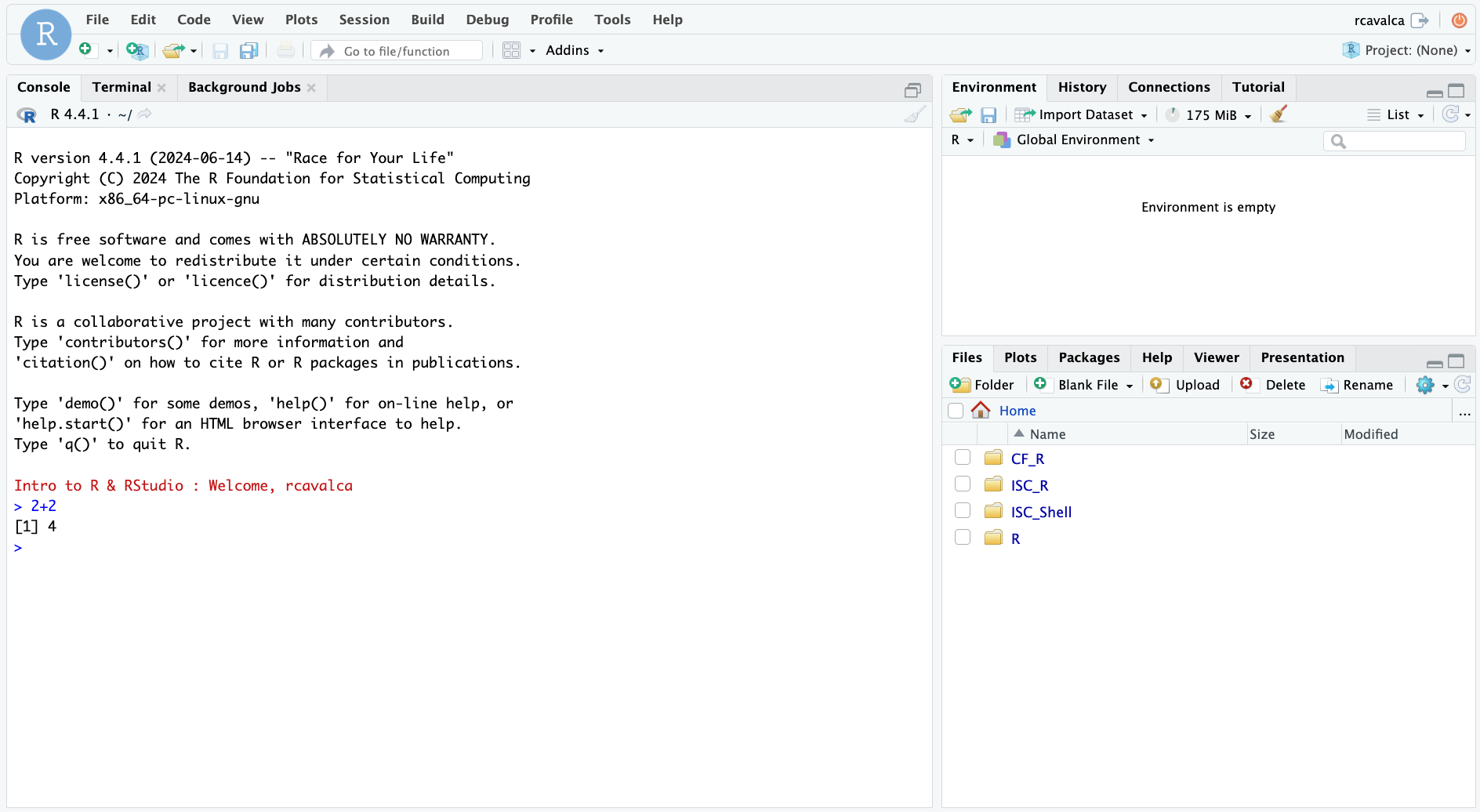

rstudio console execution

Checkpoint

Commands in a Script

Instead of entering commands directly into the Console, we’ll record them in and run them from a script. Some benefits to using a script rather than using the Console pane:

Scripts record the steps taken to analyze the data.
Scripts can be re-run, allowing for reproducibility.
Scripts are can be shared.

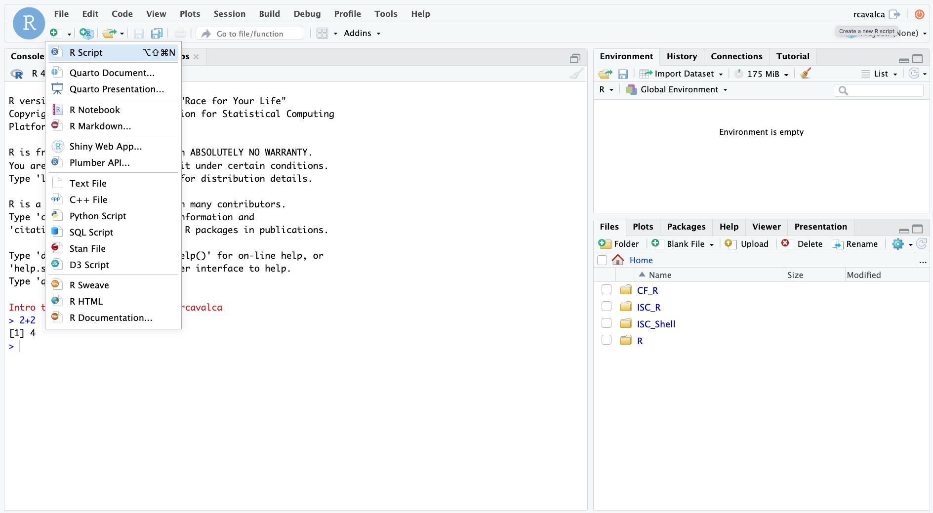
We’ll create a script file by clicking on the icon in the upper-left of the interface (a blank piece of paper with a + sign), and selecting R Script.

rstudio create script

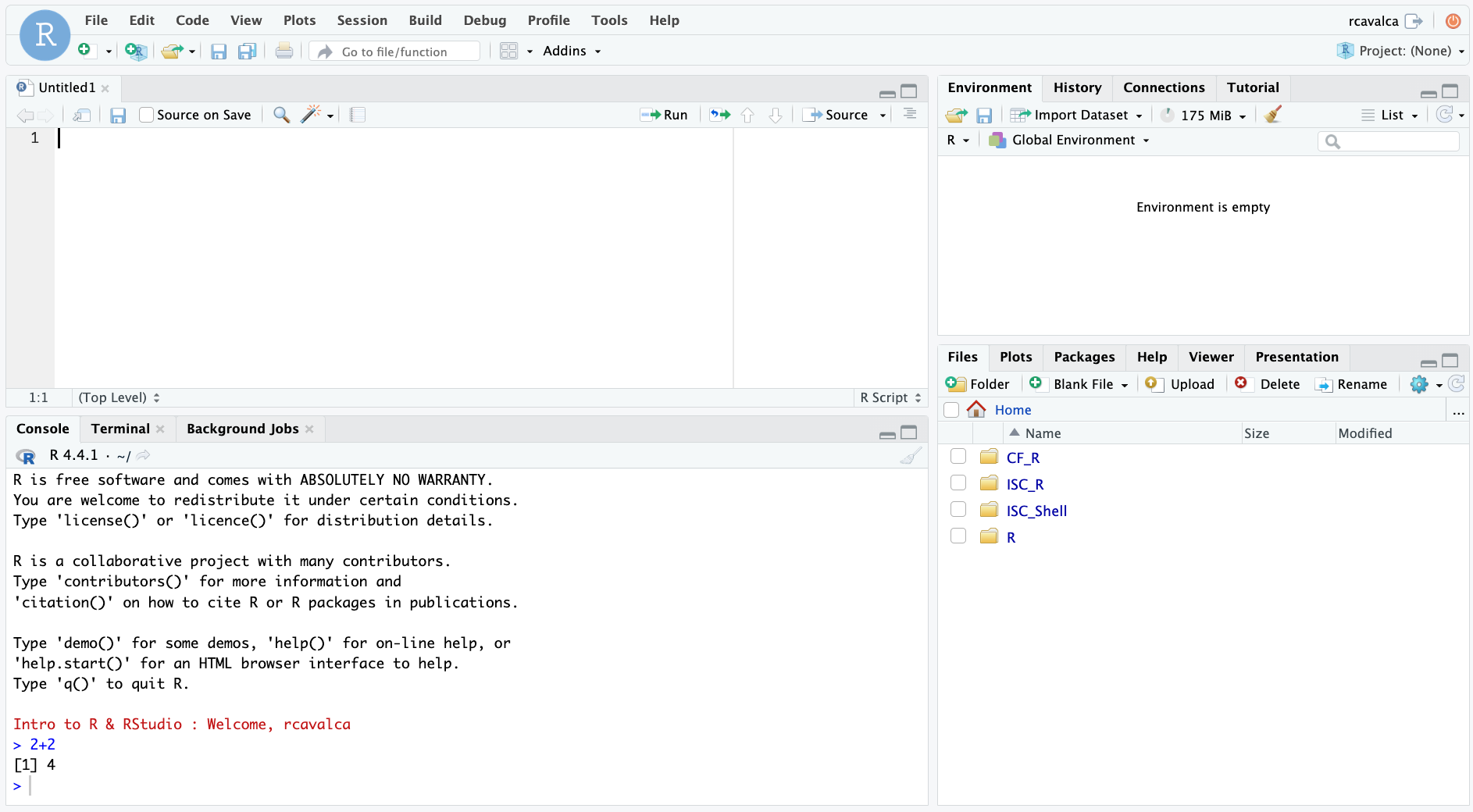
The new pane that opens is the Source pane, and you can think of it as a text editor:

rstudio script pane

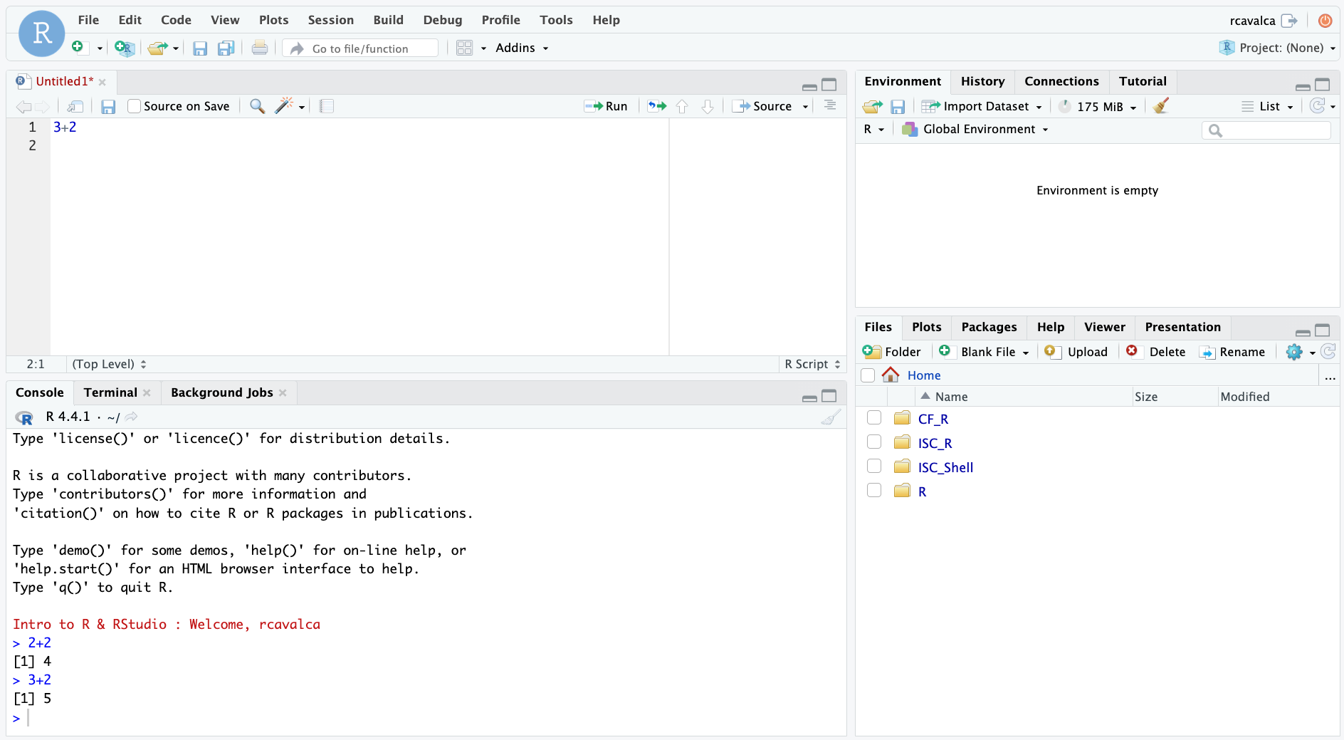
Code entered in a script file must explicitly be sent to the Console for execution with the Ctrl + Enter command. Enter the following command into the script file and execute it with Ctrl + Enter:

3+2

Looking in the Console we see the executed line and its result. Note that pressing Enter in the script creates a new line and does not execute the code as in the Console.

rstudio script execution

Console vs Script

The key differences between the Console and Script panes in RStudio:

Console	Script
Reset across sessions	Preserved acros sessions
Run with `Enter`	Run with `Ctrl + Enter`
Inconvenient to share	Convenient to share

Configuring RStudio

All of the panes in RStudio have configuration options. For example, you can minimize/maximize a pane or resize panes by dragging the borders. The most important customization options for pane layout are in the View menu. Other options such as font sizes, colors/themes, and more are in the Tools menu under Global Options.

We can enable soft-wrapping of code by selecting Code and then Soft Wrap Long Lines.

rstudio code execution

Workshop flow

To accommodate different learning styles and to keep us moving along, we’ll provide code in three different ways, and you can get that code into RStudio in corresponding ways:

Source of Code	Execution of Code
Zoom screen share	Type the code yourself.
Slack	Copy and paste into RStudio.
Website	Copy with code block button and paste into RStudio.

Questions?

Directory structure

Before we begin, the folder structure of a project organizes all the relevant files. Typically we make directories for the following types of files:

Raw data, called data, input, etc,
Results, often results or output with subfolders for tables, figures, and rdata, and
Scripts, often scripts.

We’ve already provided the raw data in the data/ folder, and it’s generally a good idea to keep raw data in its own folder.

Let’s create some folders for our analysis scripts and results thereof.

# -------------------------------------------------------------------------
# Create directory structure

dir.create('scripts', recursive = TRUE, showWarnings = FALSE)
dir.create('results/figures', recursive = TRUE, showWarnings = FALSE)
dir.create('results/tables', recursive = TRUE, showWarnings = FALSE)
dir.create('results/rdata', recursive = TRUE, showWarnings = FALSE)

Saving scripts

Let’s save our currently open script by clicking File and then Save. Double click the scripts/ folder and enter the file name ISC_day1.R.

Checkpoint

Getting started

Out of the box, R has a number of useful functions, but its power lies in extending its functionality with packages / libraries. You can think of libraries as collections of functions organized around a particular functionality. For example, the tidyverse package is a collection of packages that are designed to work together to make data manipulation and visualization easier. In order to gain access to functions in a package, we need to load the package into our R session.

Loading Libraries

Let’s begin with loading tidyverse since that’s the package we’ll use for the rest of the workshop.

# -------------------------------------------------------------------------
# Load the tidyverse package

library(tidyverse)

Note: Package loading messages

Loading a package can result in a lot of feedback from R. These aren’t necessarily errors, but give more information about the result of loading the package. The output tells us which packages were loaded (note that tidyverse is sort of a meta-package of packages). The first section of the output states which packages were lodaed and their versions. The second section notes “Conflicts” that occur because the name of a function is used multiple times. So dplyr::filter() masks stats::filter() means that the dplyr library and the stats library have functions called filter(), and that when calling filter(), the dplyr version will be the default.

Checkpoint

Loading a csv file

Let’s jump right in and load some of the gapminder data using the read_csv() function:

# -------------------------------------------------------------------------
# Load the gapminder 1997 data

gm97 = read_csv('data/gapminder_1997.csv')

Rows: 142 Columns: 6
── Column specification ───────────────────────────────────────────────────────────────────────────────────────────────────────────────────────────────────────────────────────────────────────────────────────────────────────────────────────
Delimiter: ","
chr (2): country, continent
dbl (4): year, pop, lifeExp, gdpPercap

ℹ Use `spec()` to retrieve the full column specification for this data.
ℹ Specify the column types or set `show_col_types = FALSE` to quiet this message.

Remember, with the cursor on this line we can click Run, or we can type Ctrl+Enter. We should see some output in the Console pane as well as gm97 in the Environment pane. We’ll explore the resulting data in later lessons.

Checkpoint

Let’s break down this command:

gm97 is the variable name we’re giving to the data we read in.
= is the assignment operator which assigns the object on the right to the name on the left.
read_csv() is a function in tidyverse that reads CSV files.
data/gapminder_1997.csv is the argument to read_csv() that specifies the file to read.

The output of read_csv() in the Console pane gives information such as the dimensions of the data, the delimiter of the file, and how the columns of the data were interpreted.

Note: The assignment operator

You may have seen another assignment operator, <-, which is idiosyncratic to R. We leave as an exercise to the learner to look up the edge cases of when to use <- vs =. For now, we will use = as the assignment operator, which is more common in other programming languages.

Basic R data types

In the output of read_csv(), the country and continent columns were intepreted as character strings (chr) and the year, pop, lifeExp, and gdpPercap columns were interpreted as numbers (dbl). This begs the question of the data types available in R. The basic data types in R are:

Mode (abbreviation)	Type of data	Example
Numeric (num)	Decimals, integers, etc.	`1.0`, `3.14`, `-2.5`, `10`, etc.
Character (chr)	Sequence of letters or numbers.	`"Hi"`, `'Hi'`, `"1"`, etc.
Factor (fct)	Categorical values.	Months of the year.
Logical	Boolean values	`TRUE`, `FALSE`, `T`, `F`, etc.

Assigning values to objects

Throughout this workshop we’ll be assigning names to objects and manipulating them. The names we give to objects can either make our lives easier or harder. Let’s start by describing good practices, and then we’ll give some examples of bad practices.

The good

Use brief, descriptive names.
Separate words with underscores.

# -------------------------------------------------------------------------
# Examples of good variable names, and writing over an existing variable

age = 26
age

[1] 26

wizard_name = 'Tom Riddle'
wizard_name

[1] "Tom Riddle"

wizard_name = 'Harry Potter'
wizard_name

[1] "Harry Potter"

The bad

No spaces.
Don’t start with numbers.
Don’t use proteted names, like if, else, for, etc. (see here for complete list).

# -------------------------------------------------------------------------
# Error: Example of variable name with space

favorite number = 12

Error in parse(text = input): <text>:4:10: unexpected symbol
3: 
4: favorite number
            ^

# -------------------------------------------------------------------------
# Error: Example of variable name beginning with number

1number = 3

Error in parse(text = input): <text>:4:2: unexpected symbol
3: 
4: 1number
    ^

Be mindful

Object names are case-sensitive. This means that name, Name, and NAME are three distinct objects. Imagine what confusion you could create!
Words in object names can also be separated by camelCase (e.g. objectName), but be consistent.

# -------------------------------------------------------------------------
# Example of case-sensitivity of variable names

Flower = 'marigold'
Flower

[1] "marigold"

flower = 'rose'
flower

[1] "rose"

# -------------------------------------------------------------------------
# Example of camelCase variable name

favoriteNumber = 12
favoriteNumber

[1] 12

Notice that with each assignment, the object appears in the Environment pane. Also notice that by assigning wizard_name twice, the value becomes the last assigned value, overwriting our initial assignment. Also notice that if we evaluate the name of an object, it is printed in the Console pane. We will use this pattern repeatedly.

Checkpoint

Calling functions

Earlier we ran the code gm97 = read_csv('data/gapminder_1997.csv'). As we said before, read_csv() is a function and 'data/gapminder_1997.csv' is an argument to that function. What happens if we just do:

# -------------------------------------------------------------------------
# Example of a function that needs arguments to function

read_csv()

Error in read_csv(): argument "file" is missing, with no default

We get an error in the Console pane. The key part of the message is “argument ‘file’ is missing, with no default”. In other words, this function needs to be told what to read because there is no default.

Not every function needs arguments, but many do. Try the following functions:

# -------------------------------------------------------------------------
# Examples of functions with no required arguments
Sys.Date()

[1] "2025-10-03"

getwd()

[1] "/home/workshop/rcavalca/workshop-intro-r-rstudio/source"

# -------------------------------------------------------------------------
# Example of a function with multiple arguments
round(3.1415, 2)

[1] 3.14

Notice that we threw in round() which actually takes two arguments. How could we have known that?

Getting help with functions

When a function is unfamiliar, we’ll often look at the manual page for the function to understand what arguments are required, what it does, and what it outputs. By prepending a ? in front of a function name, you can access the manual page.

# -------------------------------------------------------------------------
# Put a "?" in front of a function to see it's manual page

?round

The help page for round() tells us the function does essentially what we’d expect, and gives some other related functions. Note also that the arguments section gives us the names of the arguments and what is expected of them. There is often a Details section to describe nuances, and a Value section to describe the output. Finally, there is an Examples section which gives examples of how to run the code.

Arguments

When we called round(3.1415, 2) it seemed like the first argument is the thing we want to round, and the second argument is how many digits we want. That tracks when we look at ?round. R can evaluate arguments of a function based on their position, as we just saw. However, the preferred way to call a function is to use the names of the arguments, as in:

# -------------------------------------------------------------------------
# Example of named arguments

round(x = 3.14159, digits = 2)

[1] 3.14

Calling a function, and using named arguments, increases the readability of the code and reduces the chance of error, especially with complex functions having many arguments.

Searching for functions

Prepending a ? in front a function name to find out more about the function requires knowing the name of the function beforehand. That won’t always be the case so there are a couple ways to search for R functions.

Search the internet for “R function that does X”.
Use help.search(), as in help.search('Chi-squared test')

Note that in the results of help.search() we see things like, stats::chisq.test. Here the :: is R notation for package_name::function.

Checkpoint

Errosr happn

We already assigned some variables that resulted in errors. There will be plenty of more of those to come; they’re a normal part of coding and they are an opportunity to learn! To that end, let’s make some mistakes together.

# -------------------------------------------------------------------------
# Example of not closing quotes

read_csv('data/gapminder_1997.csv)

# -------------------------------------------------------------------------
# Example of not closing parentheses

round(3.1415, 2

In both cases, the Console displays a + to indicate that R is waiting for more input. To get out of this state, we can press Esc, and try again.

Handling errors

The key to correcting errors is understanding what went wrong. Sometimes R can help, while other times it seems willfully obtuse.

Immediately check the spelling of the command; most errors are caused by typos.
Read the error message to try to understand what might have gone wrong.
Check that the objects going into the function are what you expect.

If you’re still stuck as to why an error occurred (something we all encounter), reach out for help. For the workshop, please post the question in Slack with the following information:

The exact command that caused the error.
The exact error message that resulted.

This way we’ll more quickly be able to diagnose the problem.

Base R and the tidyverse

If you’ve used R before, you may have learned commands that are different what we’ll learn in this workshop. We’ll focus on functions from the tidyverse, a collection of R packages designed to work well together and and offer many features that aren’t part of a fresh install of R (that is, “base R”). Generally the tidyverse helps us write code that is easy to read and maintain, as we’ll see.

The tidyverse is geared for data in the form of tables, and it is very good at manipulating, summarizing, and visualizing such data. However, data occurs in a variety of other shapes and forms. In particular, in a bioinformatics context, the Bioconductor repository of packages utilize data types that are not tables, and therefore do not always work well with tidyverse functions. We’ll see clearer examples of this in the RNA-seq Demystified workshop, and you will undoubtedly encounter many examples in the future.

Some people ask “Should I learn tidyverse or base R?” and we think that rather than either/or, it’s better to think of both/and. Knowing base R and its approach will help in some contexts, while knowing tidyverse will help in others.

Cheatsheets!

The tidyverse packages have excellent cheatsheets that describe the functionality and usage of the packages. You can find them in RStudio by going to the “Help” menu and selecting “Cheat Sheets”. The two that will be most helpful in this workshop are “Data Visualization with ggplot2” and “Data Transformation with dplyr”.

Objectives

Introduce R and RStudio.
Learn how to read in a csv file.
Discuss object naming conventions and types.
Discuss functions and parameters.
Learn how to get help with functions.
Get comfortable with errors and asking for help.

Previous lesson	Top of this lesson	Next lesson

Introducing R and RStudio

Objectives

The gapminder dataset

Server login

Create a project

The RStudio interface

Commands in the Console

Commands in a Script

Console vs Script

Configuring RStudio

Workshop flow

Directory structure

Saving scripts

Getting started

Loading Libraries

Note: Package loading messages

Loading a csv file

Note: The assignment operator

Basic R data types

Assigning values to objects

The good

The bad

Be mindful

Calling functions

Getting help with functions

Arguments

Searching for functions

Errosr happn

Handling errors

Base R and the tidyverse

Cheatsheets!

Objectives