R Basics
Overview
In this lesson we will begin to work with objects in R, understand conventions around their use, learn about types of objects and how to alter and otherwise manipulate them. R has many different types of objects, and we will not cover all of them in depth. Instead, we will take care to introduce and work with the most common types (vectors and data frames), while introducing briefly types we won’t encounter much in this workshop (matrices, arrays, and lists).
A word of encouragement
Before we begin this lesson, we want to make clear that learning a programming language takes time. At first, things may seem unfamiliar and you may feel like you don’t have the tools to do what you want to do. Sometimes it’s easier to say in words what the intended result is, than to code it out. And that’s okay. As you spend time in R (or in other languages), you will find that you have more functions at your recall, and you will more quickly be able to implement your goals in code.
Reminder
At this point you should be coding along in the “r_basics.R” script we created in the last episode. Writing your commands and comments in the script will make it easier to record what you did and why. We should also be regularly saving the file by clicking the single floppy disk icon or typing Ctrl + S.
Creating objects
Let’s start working with R by creating our first object. Many other programming languages refer to an object as a variable, and it’s okay to use the two interchangeably.
To create an object you need:
- a name (e.g. ‘a’)
- a value (e.g. ‘1’)
- the assignment operator (‘<-’)
In your script, “r_basics.R”, using the R assignment operator ‘<-’, assign ‘1’ to the object ‘a’ as shown. Remember to leave a comment in the line above (using the ‘#’) to explain what you are doing:
# this line creates the object 'a' and assigns it the value '1'
a <- 1
Next, run this line of code in your script. In the RStudio ‘Console’ you should see:
> a <- 1
>
The ‘Console’ will display lines of code run from a script and any outputs or status/warning/error messages (usually in red).
In the ‘Environment’ window you will also get a table:
| Values | |
|---|---|
| a | 1 |
The ‘Environment’ window allows you to keep track of the objects you have created in R.
Exercise: Create some objects
Create the following objects:
- Create an object called
human_chr_numberthat has the value of number of pairs of human chromosomes- Create an object called
gene_namethat has the value of your favorite gene name
Solution
Here as some possible answers to the challenge:
human_chr_number <- 23
gene_name <- 'pten'
Comment on the assignment operator
Many people use
=as their preferred assignment operator in R instead of<-, and this is just as well. Here is a blog post discussing the differences.
Naming objects in R
The following recommendations on variable naming should keep our code readable and interpretable:
- Avoid spaces and special characters: Object names
cannot contain spaces or the minus sign (
-). You can use ’_’ to make names more readable. You should avoid using special characters in your object name (e.g. ! @ # , etc.). Also, object names cannot begin with a number. - Use short, easy-to-understand names: You should avoid naming your objects using single letters (e.g. ‘n’, ‘p’, etc.). This is mostly to encourage you to use names that would make sense to anyone reading your code (a colleague, or even yourself a year from now). Also, avoiding excessively long names will make your code more readable.
- Avoid commonly used names: There are several names that may already have a definition in the R language (e.g. ‘mean’, ‘min’, ‘max’). One clue that a name already has meaning is that if you start typing a name in RStudio and it gets a colored highlight or RStudio gives you a suggested autocompletion you have chosen a name that has a reserved meaning.
- Use the recommended assignment operator: In R, we
use ‘<-’ as the preferred assignment operator. ‘=’ works too, but is
most commonly used in passing arguments to functions (more on functions
later). There is a shortcut for the R assignment operator:
- Windows execution shortcut: Alt+-
- Mac execution shortcut: Option+-
There are a few more suggestions about naming and style you may want to learn more about as you write more R code. There are several “style guides” that have advice, and one to start with is the tidyverse R style guide.
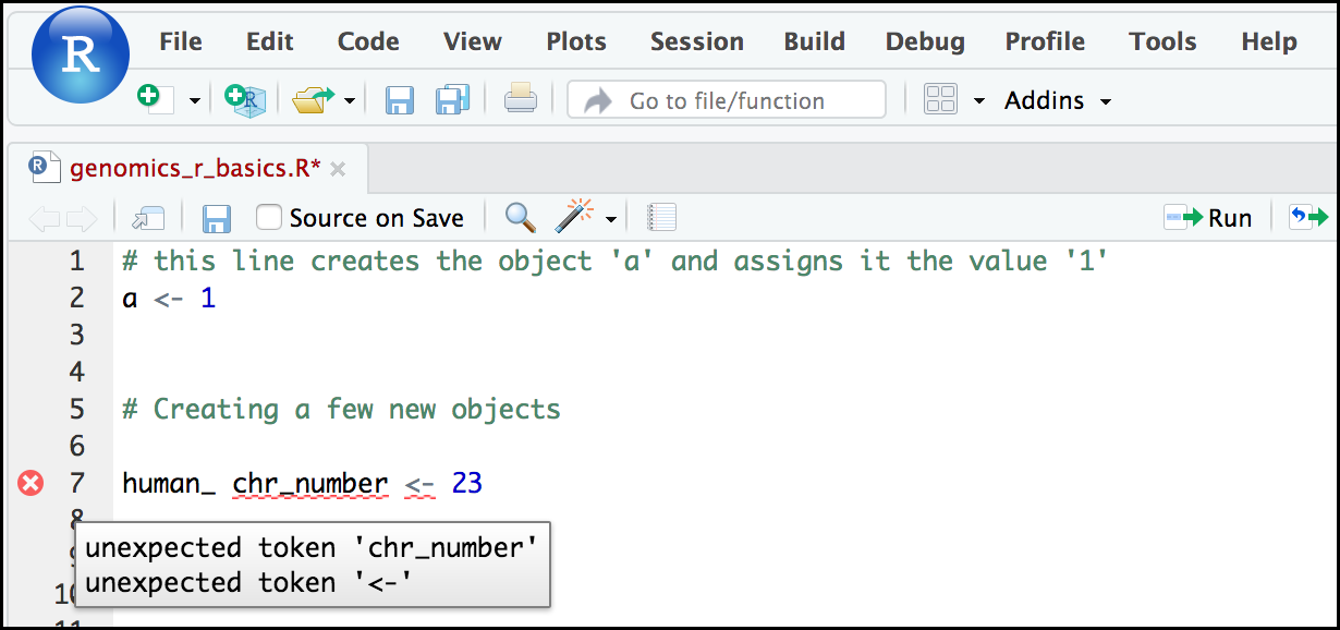
Tip: Pay attention to warnings in the script console
If you enter a line of code in your script that contains an error, RStudio may give you an error message and underline this mistake. Sometimes these messages are easy to understand, but often the messages may need some figuring out. Paying attention to these warnings will help you avoid mistakes. In the example below, our object name has a space, which is not allowed in R. The error message does not say this directly, but R is “not sure” about how to assign the name to “human_ chr_number” when the object name we want is “human_chr_number”.
Reassigning object names or deleting objects
Once an object has a value, you can change that value by overwriting it. R will not give you a warning or error if you overwriting an object, which may or may not be a good thing depending on how you look at it.
# gene_name has the value 'pten' or whatever value you used in the challenge.
# We will now assign the new value 'tp53'
gene_name <- 'tp53'
You can also remove an object from R’s memory entirely. The
rm() function will delete the object.
# delete the object 'gene_name'
rm(gene_name)
If you run a line of code that has only an object name, R will normally display the contents of that object. In this case, we are told the object no longer exists.
Error: object 'gene_name' not foundObject data types
In R, every object has two properties:
- Length: How many values are held in that object
- Mode: What is the classification (type) of that object.
We will get to the “length” property later in the lesson. The “mode” property **corresponds to the type of data an object represents. The most common modes you will encounter in R are:
| Mode (abbreviation) | Type of data |
|---|---|
| Numeric (num) | Numbers such floating point/decimals (1.0, 0.5, 3.14), there are also more specific numeric types (dbl - Double, int - Integer). These differences are not relevant for most beginners and pertain to how these values are stored in memory |
| Character (chr) | A sequence of letters/numbers in single ’’ or double ” ” quotes |
| Logical | Boolean values - TRUE or FALSE |
There are a few other modes (i.e. “complex”, “raw” etc.) but these are the three we will work with in this lesson.
Data types are familiar in many programming languages, but also in natural language where we refer to them as the parts of speech, e.g. nouns, verbs, adverbs, etc. Once you know if a word - perhaps an unfamiliar one - is a noun, you can probably guess you can count it and make it plural if there is more than one (e.g. 1 parrot, or 2 parrots). If something is an adjective, you can usually change it into an adverb by adding “-ly” (e.g. slow and slowly). Depending on the context, you may need to decide if a word is in one category or another (e.g “cut” may be a noun when it’s on your finger, or a verb when you are preparing vegetables). These concepts have important analogies when working with R objects.
Exercise: Create objects and check their modes
Create the following objects in R, then use the
mode()function to verify their modes. Try to guess what the mode will be before you look at the solution
chromosome_name <- 'chr02'scale_factor <- 0.47chr_position <- '1001701'spock <- TRUEpilot <- Earhart
Solution
chromosome_name <- 'chr02'
scale_factor <- 0.5
chr_position <- '1001701'
spock <- TRUE
pilot <- Earhart
Error in eval(expr, envir, enclos): object 'Earhart' not foundmode(chromosome_name)[1] "character"mode(scale_factor)[1] "numeric"mode(chr_position)[1] "character"mode(spock)[1] "logical"mode(pilot)Error in mode(pilot): object 'pilot' not foundNotice that R interprets a series of numbers wrapped in quotes as
being in “character” mode. Also notice that
pilot <- Earhart gave an error. This is because, without
the quotes, R expected Earhart to be an object, but there
is no such named object yet. If Earhart did exist, then the
mode of pilot would be whatever the mode of
Earhart was originally. If we did indeed want
pilot to be assigned the name “Earhart” we would do:
pilot <- "Earhart"
mode(pilot)
[1] "character"Mathematical and functional operations on objects
Once an object exists (and by definition has a mode), R can appropriately manipulate that object. For example, objects of the numeric modes can be added, multiplied, divided, etc. R provides several mathematical (arithmetic) operators including:
| Operator | Description |
|---|---|
| + | addition |
| - | subtraction |
| * | multiplication |
| / | division |
| ^ or ** | exponentiation |
| a%/%b | integer division (division where the remainder is discarded) |
| a%%b | modulus (returns the remainder after division) |
These can be used with literal numbers:
(1 + (5^0.5))/2[1] 1.618034and importantly, can be used on any object that evaluates to (i.e. interpreted by R) a numeric object:
# multiply the object 'human_chr_number' by 2
human_chr_number * 2
[1] 46Vectors
Vectors are probably the most commonly used object type in R.
A vector is a collection of values that are all of the same type
(numbers, characters, etc.). One of the most common ways to
create a vector is to use the c() function - the
“concatenate” or “combine” function. Inside the function you may enter
one or more values; for multiple values, separate each value with a
comma:
# Create a vector of country names
countries <- c("Thailand", "Lesotho", "Suriname", "Canada")

# Continent of country
continents <- c('Asia', 'Africa', 'South America', 'North America')

# Population of country
populations <- c(69950850, 2108328, 575990, 38436447) # Source: Wikipedia

# Logical vector of Asian countries
on_asia <- c(TRUE, FALSE, FALSE, FALSE)
Vectors always have a mode and a
length. You can check these with the
mode() and length() functions respectively.
Another useful function that gives both of these pieces of information
is the str() (structure) function.
# Check the mode, length, and structure of 'countries'
mode(countries)
[1] "character"length(countries)[1] 4str(countries) chr [1:4] "Thailand" "Lesotho" "Suriname" "Canada"mode(continents)[1] "character"mode(populations)[1] "numeric"mode(on_asia)[1] "logical"Vectors are quite important in R. Another data type that we will work with later in this lesson, data frames, are collections of vectors. What we learn here about vectors will pay off even more when we start working with data frames.
Creating and subsetting vectors
Once we have vectors, it is common to want to need to extract one or more values from them. We bracket notation to do this. We type the name of the vector followed by square brackets. In those square brackets we place the index (e.g. a number) in that bracket as follows:
# get the 3rd value in the countries vector
countries[3]
[1] "Suriname"In R, every item in a vector is indexed, starting from the first item (1) through the final number of items in your vector. You can also retrieve a range of numbers:
# get the 1st through 3rd value in the countries vector
countries[1:3]
[1] "Thailand" "Lesotho" "Suriname"If you want to retrieve several (but not necessarily sequential) items from a vector, you pass a vector of indices; a vector that has the numbered positions you wish to retrieve.
# get the 1st, 3rd, and 4th value in the countries vector
countries[c(1, 3, 4)]
[1] "Thailand" "Suriname" "Canada" If you want to use a logical vector to retrieve only the Asian countries you can do the following. We will see other ways of logically subsetting vectors in a bit.
# Get the Asian countries
countries[on_asia]
[1] "Thailand"There are additional (and perhaps less commonly used) ways of subsetting a vector (see these examples). Also, several of these subsetting expressions can be combined:
# get the 4th value, and then the 1st through the 3rd value
# in other words, you can reorder the countries
countries[c(4, 1:3)]
[1] "Canada" "Thailand" "Lesotho" "Suriname"Adding to, removing, or replacing values in existing vectors
Once you have an existing vector, you may want to add a new item to
it. To do so, you can use the c() function again to add
your new value:
# add the countries 'Bolivia' and 'Tonga' to our list of countries
# this overwrites our existing vector
countries <- c(countries, "Bolivia", "Tonga")
We can verify that “countries” contains the new entries
countries[1] "Thailand" "Lesotho" "Suriname" "Canada" "Bolivia" "Tonga" Using a negative index will return a version of a vector with that index’s value removed:
countries[-6][1] "Thailand" "Lesotho" "Suriname" "Canada" "Bolivia" We can remove that value from our vector by overwriting it with this expression:
countries <- countries[-6]
countries
[1] "Thailand" "Lesotho" "Suriname" "Canada" "Bolivia" We can also explicitly rename or add a value to our index using bracket notation:
countries[7]<- "Estonia"
countries
[1] "Thailand" "Lesotho" "Suriname" "Canada" "Bolivia" NA "Estonia" Notice in the operation above that R inserts an NA value
to extend our vector so that the country “Estonia” is in index 7. This
may be a good or not-so-good thing depending on how you use this.
Exercise: Working with vectors
- How do we extract the third element of the
countriesvector?- How do we get the length of the
countriesvector?- What function can concatenate other values onto a vector?
- How could we multiply all the populations by 2?
Solution
countries[3]length(countries)c()populations * 2
Logical Subsetting
We saw with countries[on_asia] that we could use a
literal logical vector in the bracket notation to extract the
TRUE indices of a vector. But we can also use a logical
expression. Let’s say we wanted get all of the countries in our vector
of country populations that were less than 10,000,000. We could index
using the ‘<’ (less than) logical operator:
# Subset populations to those less than 10 million
populations[populations < 10000000]
[1] 2108328 575990In the square brackets we essentially write an expression for a
logical test of the vector. In this case
populations < 10000000, which R will then evaluate into
a logical vector. Some of the most common logical operators you will use
in R are:
| Operator | Description |
|---|---|
| < | less than |
| <= | less than or equal to |
| > | greater than |
| >= | greater than or equal to |
| == | exactly equal to |
| != | not equal to |
| !x | not x |
| a | b | a or b |
| a & b | a and b |
There is a related way of doing this which returns the indices which
are TRUE, using the which() function.
which(populations < 10000000)[1] 2 3And then subsetting populations with the above expression in the square brackets gives the same result:
# Subset populations to those less than 10 million
populations[which(populations < 10000000)]
[1] 2108328 575990Finally, a useful idea is to replace the hard-coded 10,000,000 with a variable. Often we won’t know what inputs and values will be used when our code is executed, so we could also do something like:
pop_thresh = 10000000
populations[populations < pop_thresh]
[1] 2108328 575990And if we were to use that pop_thresh multiple times in
our code, and wanted to change it, we’d only have to change one location
rather than many, thus reducing errors.
A few final vector tricks
There are a few other common retrieve or replace operations you may
want to know about. First, you can check to see if any of the values of
your vector are missing (i.e. are NA). The
is.na() function will return a logical vector, with TRUE
for any NA value:
# current value of 'countries':
# chr [1:7] "Thailand" "Lesotho" "Suriname" "Canada" "Bolivia" NA "Estonia"

is.na(countries)
[1] FALSE FALSE FALSE FALSE FALSE TRUE FALSESometimes, you may wish to find out if a specific value (or several
values) is present a vector. You can do this using the comparison
operator %in%, which will return TRUE for any value in your
collection that is in the vector you are searching:
# current value of 'countries':
# chr [1:7] "Thailand" "Lesotho" "Suriname" "Canada" "Bolivia" NA "Estonia"

# test to see if "Lesotho" or "Canada" is in the countries vector
# if you are looking for more than one value, you must pass this as a vector
c("Lesotho", "Canada") %in% countries
[1] TRUE TRUEReview Exercise 1
Add the following values to the specified vectors:
- To the
continentsvector add: “South America”- To the
populationsvector add: 11428245
Solution
continents <- c(continents, "South America") # did you use quotes?
continents
[1] "Asia" "Africa" "South America" "North America"
[5] "South America"populations <- c(populations, 11428245)
populations[1] 69950850 2108328 575990 38436447 11428245Review Exercise 2
Using indexing, create a new vector named
combinedthat contains:
- The the 1st value in
countries- The 1st value in
continents- The 1st value in
populations
Solution
combined <- c(countries[1], continents[1], populations[1])
combined
[1] "Thailand" "Asia" "69950850"Review Exercise 3
What type of data is
combined? Why?
Solution
typeof(combined)[1] "character"Data reset
Before we continue, let’s reset some vectors:
# Create a vector of country names
countries <- c("Thailand", "Lesotho", "Suriname", "Canada")

# Continent of country
continents <- c('Asia', 'Africa', 'South America', 'North America')

# Population of country
populations <- c(69950850, 2108328, 575990, 38436447) # Source: Wikipedia

# Logical vector of Asian countries
on_asia <- c(TRUE, FALSE, FALSE, FALSE)
Bonus material: Matrices and Lists
Matrices
A matrix stores values in a two-dimensional array, as in a matrix
from linear algebra. A matrix must store data that is all the same type.
We can create a matrix from a vector by using the matrix()
function and specifying the number of rows (or columns), as with:
country_matrix = matrix(countries, nrow = 2)
country_matrix
[,1] [,2]
[1,] "Thailand" "Suriname"
[2,] "Lesotho" "Canada" mode(country_matrix)[1] "character"class(country_matrix)[1] "matrix" "array" dim(country_matrix)[1] 2 2Notice that since a matrix has two-dimensions, it’s “length” should
really be thought of as dimensions, i.e. the number of rows and columns
(in that order with dim()). To access entires of a matrix,
we also use bracket notation. Some examples of accessing specific
entries:
# Return the element in the first row, second column
country_matrix[1, 2]
[1] "Suriname"# Return the element in the second row, second column
country_matrix[2, 2][1] "Canada"If we wanted to return a whole row, or a whole column, we would leave the row or column entry blank, respectively, as in:
# Return the first row
country_matrix[1, ]
[1] "Thailand" "Suriname"# Return the second column
country_matrix[, 2][1] "Suriname" "Canada" Lists
Lists are like vectors in that they group data into a one-dimensional set, but lists group together other R objects, such as vectors or other lists. The best way to see this is with an example:
country_list = list(countries, continents, populations)
country_list
[[1]]
[1] "Thailand" "Lesotho" "Suriname" "Canada"
[[2]]
[1] "Asia" "Africa" "South America" "North America"
[[3]]
[1] 69950850 2108328 575990 38436447mode(country_list)[1] "list"length(country_list)[1] 3Notice that the list contains three vectors, the types of the vectors don’t have to be the same. In fact, the length of the vectors don’t even have to be the same.
To access the first element of country_list and
return a list, we would use the single-bracket
notation:
country_list[1][[1]]
[1] "Thailand" "Lesotho" "Suriname" "Canada" mode(country_list[1])[1] "list"If we wanted to access the first element and return an atomic vector, we would use double-bracket notation:
country_list[[1]][1] "Thailand" "Lesotho" "Suriname" "Canada" mode(country_list[[1]])[1] "character"Tip: Where to learn more
The following are good resources for learning more about R. Some of them can be quite technical, but if you are a regular R user you may ultimately need this technical knowledge.
- R for Beginners: By Emmanuel Paradis and a great starting point
- The R Manuals: Maintained by the R project
- R contributed documentation: Also linked to the R project; importantly there are materials available in several languages
- R for Data Science: A wonderful collection by noted R educators and developers Garrett Grolemund and Hadley Wickham
- Practical Data Science for Stats: Not exclusively about R usage, but a nice collection of pre-prints on data science and applications for R
- Programming in R Software Carpentry lesson: There are several Software Carpentry lessons in R to choose from