DE Initialization

In this module, we will learn:

• How to ‘unblind’ our samples
• How to ensure high quality count data with filtering

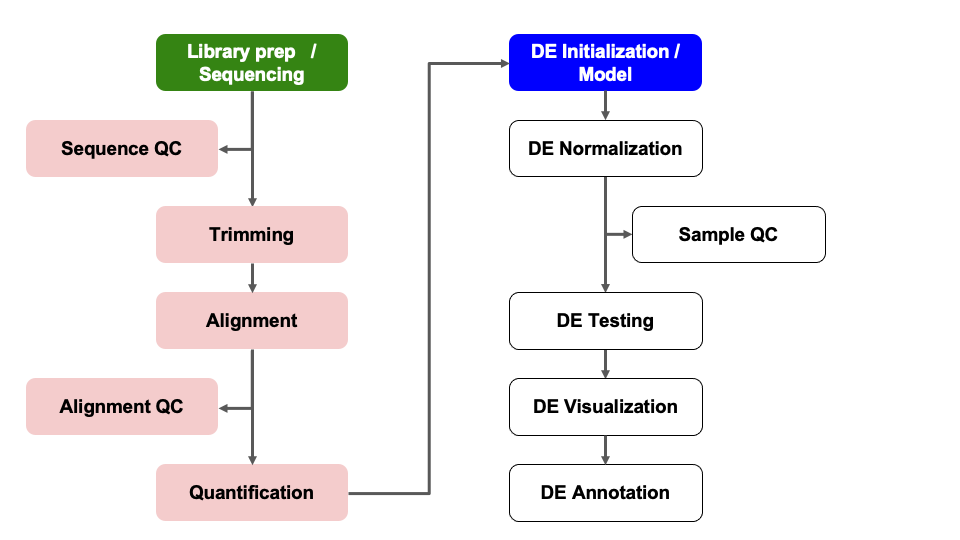
Differential Expression Workflow

Here we will setup the inputs needed to initialize DESeq2 before testing for differential expression.

---

Sample Information

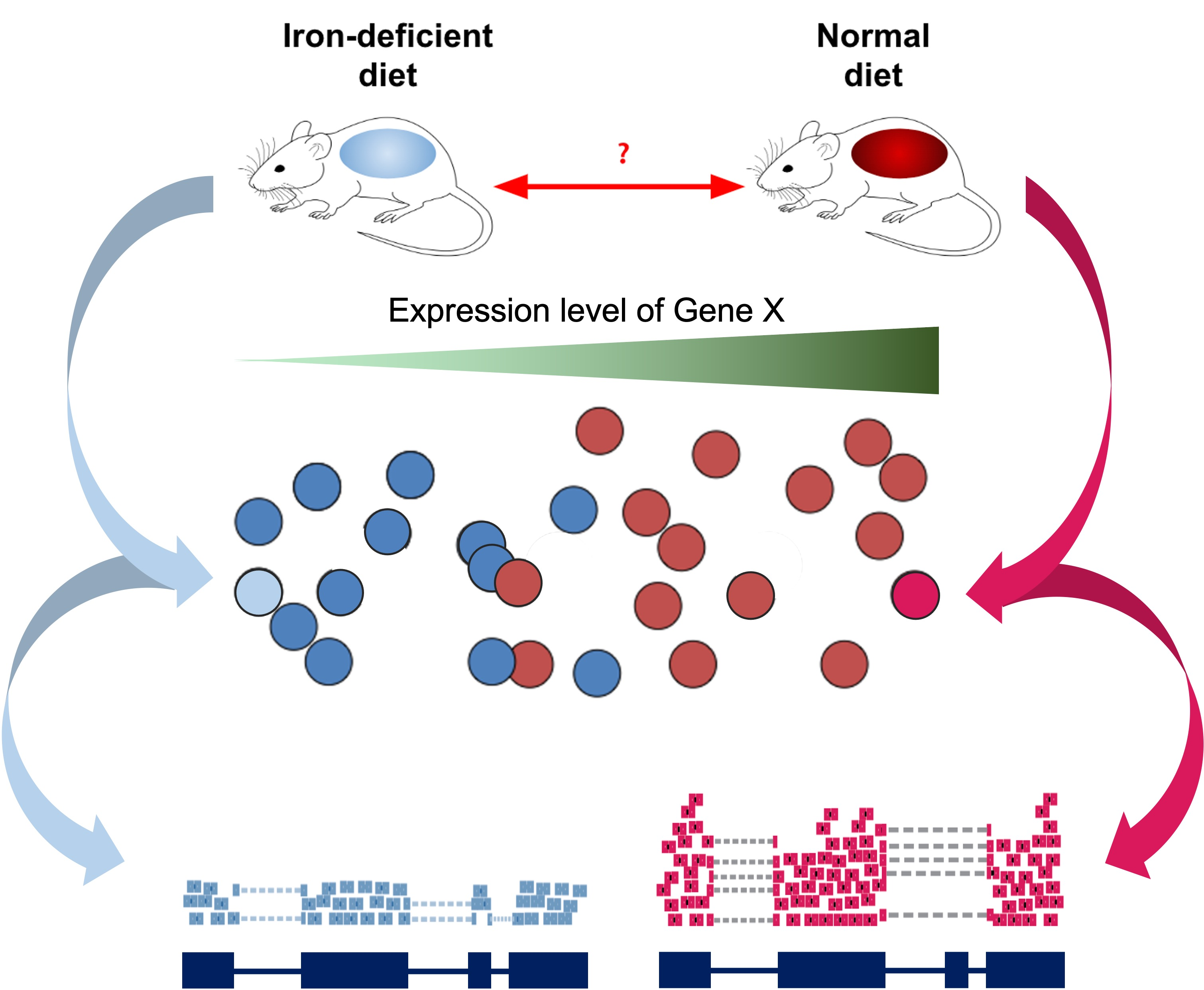
As introduced at the beginning of the workshop, we have downloaded and prepared data from an existing publication (Zhang et al., 2019), wherein one goal is to understand the gene expression differences in wild-type mice that that were “iron replete” and fed a control diet (we label these “control”) and “iron deficient” (we label these “deficient”).

Read Sample Table

Our next step will be to describe the samples within our R session, so that we make the proper comparisons with DESeq2. Let’s check the sample names from the count table.

colnames(count_table)

[1] "sample_A" "sample_B" "sample_C" "sample_D" "sample_E" "sample_F"

Based on the sample names that are the columns of count_table, our samples are blinded, e.g. the sample names don’t clearly correspond to treatment groups. We will need to specify which sample IDs connect to which experimental conditions.

Typically sample phenotype data, including experimental conditions, are stored as Excel or CSV files that we can read into R, and then use when creating a DESeq2 object. If you are unfamilar with CSV files or how to generate them, there are tutorials available to guide you through the process.

Tip: Sample naming conventions

Use only alpha-numeric characters (A-Z, a-z, 0-9), and separate parts of the name with underscores (_) or dots (.). Do not begin sample names with numbers.

We’ll load our ‘pre-made’ sample information sheet, samplesheet.csv, to unblind our samples.

samplesheet = read.table("data/samplesheet.csv",
                       sep = ",",
                       header = TRUE,
                       row.names = 1)

Alternatively, we could manually create a sample sheet, ensuring that the sample IDs match our count table.

We can look at the object by typing its name and hitting Enter. Note, for larger experiments, you may want to use head().

samplesheet

         genotype condition
sample_A       wt   control
sample_B       wt   control
sample_C       wt   control
sample_D       wt deficient
sample_E       wt deficient
sample_F       wt deficient

Checkpoint: If you have loaded samplesheet, please indicate with the green ‘check’ button. Otherwise, please use the red ‘x’ button to have the command repeated

In this example data, all mice are of a wild-type genotype with three samples from control diet mice (labeled as “control”) and three samples from iron deficient diet fed mice (labeled as “deficient”). Again, for larger experiments, you may want to examine the coding of the samples and how many group labels are present by looking at the unique() values of the relevant columns.

unique(samplesheet$condition)

[1] "control"   "deficient"

Replicates and sequencing depth in RNA-seq experiments

Question In this experiment, we only have samples from three mice per each condition. Do we have enough replicates?

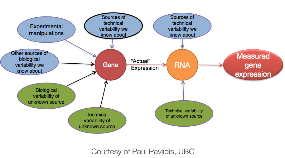
The goal of our analysis is to separate the “interesting” biological contributions from the “uninteresting” technical or other contributions that either cannot be or were not controlled in the experimental design. The more sources of variation, such as samples coming from heterogenous tissues or experiments with incomplete knockdowns, the more replicates (>3) are recommended.

Image of technical, biological, and experimental contributors to gene expression, from HBC training materials

For a more in depth discussion of experimental design considerations, particularly for the number of replicates, please read A Beginner’s Guide to Analysis of RNA Sequencing Data or papers like this one by Hart et al that focus on estimating statistical power for RNA-seq experiments.

Sample table formatting

Next, we’ll format our table so that we have the appropriate data type (an ordered factor) for DESeq2 to recognize our treatment groups and appropriately compare samples.

# tidy version
samplesheet_ready <- samplesheet %>% mutate(condition = factor(condition, 
                                          levels = c('control', 'deficient')))

# base version
samplesheet_ready <- samplesheet
samplesheet_ready$condition = factor(samplesheet_ready$condition,
                            levels = c('control', 'deficient'))

unique(samplesheet_ready$condition)

[1] control   deficient
Levels: control deficient

Notice that we set the levels in a particular order. This is important for setting the “Control” (or “Reference”) group as the denominator in the default comparisons when we setup our DESeq2 model.

Before we proceed, we need to make sure that the sample labels (column names) in the count table match the sample information table (row names), including the order. If the sample labels don’t match, then we will see an error and need to correct the labels prior to proceeding. Checking the sample information table is extremely important to ensure that the correct samples are grouped together for comparisons.

all(colnames(count_table) == rownames(samplesheet_ready))

[1] TRUE

This line of code checks if both the identity and order match between our count_table and our samplesheet. If, in the course of using your own data, this returns FALSE, try using the match() function to rearrange the columns of count_table (or the rows of samplesheet) to get them to match.

Checkpoint: If you your sample info check returns TRUE, please indicate with the green ‘yes’ button. Otherwise, please use the red ‘x’ button to have the command repeated

Creating DESeq2 object

Bioconductor software packages often define and use custom structures to store data in a way that suits biological data, such as illustrated below from Huber et al. 2015.

A breakdown of the SummarizedExperiment class.

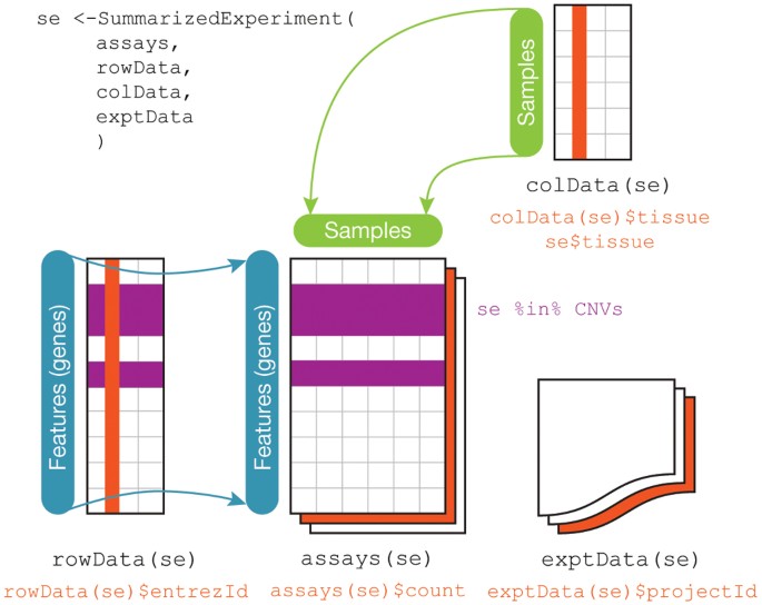
These custom data structures have pre-defined data slots, which hold specific types/classes of data and therefore can be more easily accessed by functions from the same package.

To create the DESeqDataSet we need two important inputs:

1. A table that assigns the condition labels for each sample (that we read in and formatted)
2. A raw count matrix

Is our count matrix from our RSEM outputs considered a “raw” count matrix by DESeq2?

If we think back to the RSEM outputs, the ‘expected_counts’ table may include fractional amounts due to how the alignment tool resolves reads mapping to multiple locuses). However, recent versions of DESeq2 handle this without rounding.

To create the DESeqDataSet we will need the count_table and the samplesheet. We will also need a design formula to specify our model.

Making model choices

We’ll talk about the design formula more later but for now it’s important to understand that the design specifies the relevant column(s) in the metadata table and how they should be used when fitting a model for our data.

For our dataset we only have one column we are interested in, that is condition. This column has two factor levels, which tells DESeq2 that for each gene we want to evaluate gene expression change with respect to these different levels. Although the design formula is required, it is not used at this step.

## Create DESeq object, line by line
dds = DESeqDataSetFromMatrix(countData = count_table,
                              colData = samplesheet_ready,
                              design = ~ condition)
dds

class: DESeqDataSet 
dim: 55492 6 
metadata(1): version
assays(1): counts
rownames(55492): ENSMUSG00000000001 ENSMUSG00000000003 ... mcherry tdtomato
rowData names(0):
colnames(6): sample_A sample_B ... sample_E sample_F
colData names(2): genotype condition

Notice that printing the dds object helpfully shows us some helpful information:

• The dimension (number of genes by number of samples),
• The gene identifiers,
• The sample identifiers,
• The additional column names giving information about the samples

Checkpoint: If you see dds in your environment panel, please indicate with the green ‘check’ button. Otherwise, please use use the red ‘x’ button in your zoom reaction panel to have this step repeated. You can use the red ‘x’ to be put in a breakout room for help

---

Pre-filtering

While not necessary, pre-filtering helps to not only reduce the size of the DESeq2 object, but also gives you a sense of how many genes were reasonably measured at the sequencing depth generated for your samples.

Here we will filter out any genes that have less than 10 counts across any of the samples. This is a fairly standard level of filtering, but can filter data less/more depending on quality control metrics from alignments and sequencing depth or total number of samples.

keep = rowSums(counts(dds)) >= 10
dds_filtered = dds[keep,]
dds_filtered

class: DESeqDataSet 
dim: 16249 6 
metadata(1): version
assays(1): counts
rownames(16249): ENSMUSG00000000001 ENSMUSG00000000028 ... ENSMUSG00000118651 ENSMUSG00000118653
rowData names(0):
colnames(6): sample_A sample_B ... sample_E sample_F
colData names(2): genotype condition

Notice the dds_filtered object has less elements than the unfiltered dds object, indicating that a number of genes were not measured in our experiment.

Checkpoint: Questions?

Summary

In this section, we:

• Loaded the necessary input files into our R session
• Discussed single variable model design for DESeq2
• Initialized a DESeq2 data set
• Filtered our count data

Now that we’ve created our DESeq2 objects, including specifying what model is appropriate for our data, and filtered our data, we can proceed with assessing the impact of the experimental conditions on gene expression for our samples.

---

Sources

Training resources used to develop materials:

• HBC DGE setup: https://hbctraining.github.io/DGE_workshop/lessons/01_DGE_setup_and_overview.html
• HBC Count Normalization: https://hbctraining.github.io/DGE_workshop/lessons/02_DGE_count_normalization.html
• DESeq2 standard vignette: http://bioconductor.org/packages/devel/bioc/vignettes/DESeq2/inst/doc/DESeq2.html
• DESeq2 beginners vignette: https://bioc.ism.ac.jp/packages/2.14/bioc/vignettes/DESeq2/inst/doc/beginner.pdf
• Bioconductor RNA-seq Workflows: https://www.bioconductor.org/help/course-materials/2015/LearnBioconductorFeb2015/B02.1_RNASeq.html
• CCDL Gastric cancer training materials: https://alexslemonade.github.io/training-modules/RNA-seq/03-gastric_cancer_exploratory.nb.html
• CCDL Neuroblastoma training materials: https://alexslemonade.github.io/training-modules/RNA-seq/05-nb_cell_line_DESeq2.nb.html

---

These materials have been adapted and extended from materials listed above. These are open access materials distributed under the terms of the Creative Commons Attribution license (CC BY 4.0), which permits unrestricted use, distribution, and reproduction in any medium, provided the original author and source are credited.

---

Previous lesson	Top of this lesson	Next lesson