DE Normalization

In this module, we will learn:

• Different count normalizations and their uses
• How to fit a model for differential expression comparisons

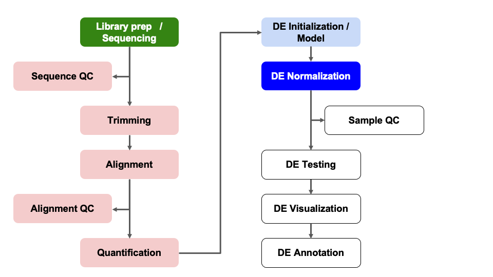
Differential Expression Workflow

Here we will proceed with count normalizations.

---

Count normalizations

Since counts of mapped reads for each gene is proportional to the expression of RNA in addition to many “uninteresting” other factors, normalization is the process of scaling raw count values to account for the “uninteresting” factors and ensure expression levels are more comparable.

Normalization goals

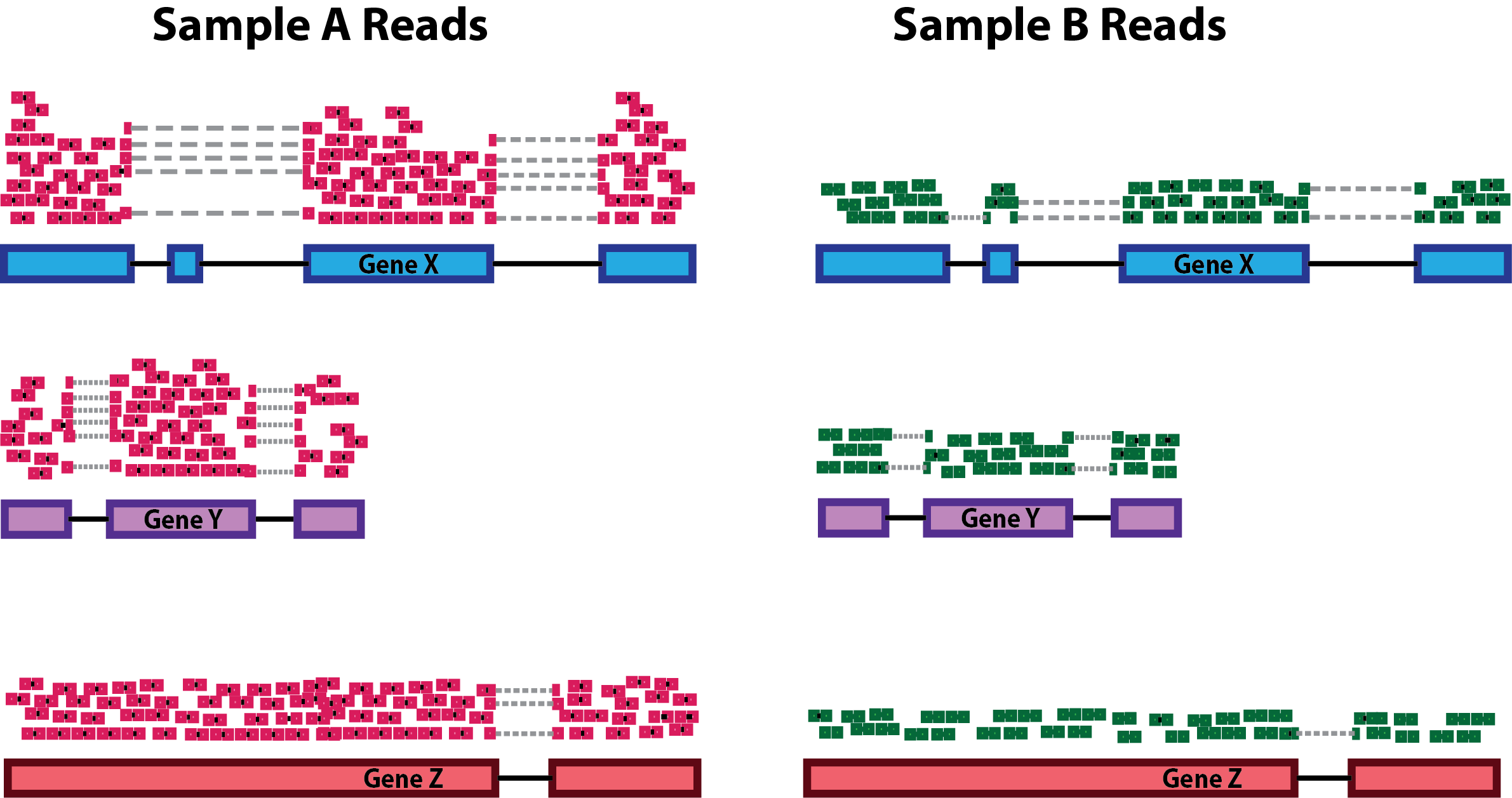
Two common factors that need to be accounted for during normalization are sequencing depth and gene length. Common normalization approaches (such as FPKM, RPKM, CPM, TPM, etc.) account for one or both of these factors.

• Sequencing depth normalization is necessary to account for the proportion of reads per gene expected for more deeply sequenced samples (like in pink below) versus a less deeply sequenced sample (like in green below).

Note that each pink or green rectangle represents an aligned read, with reads spanning an intron connected by a dashed line. Figure from HBC training materials

• Gene length normalization may also be necessary if comparing between different genes, since genes of different lengths have different probabilities of generating fragments that end up in the library.

Note: The above figure was originally from a HBC tutorial that also includes a detailed comparison of different normalization (CPM, TPM, FPKM) approaches and their best uses, which are summarized below.

Common normalization methods

Several common normalization methods exist to account for these differences:

Normalization method	Description	Accounted factors	Recommendations for use
CPM (counts per million)	counts scaled by total number of reads	sequencing depth	gene count comparisons between replicates of the same samplegroup; NOT for within sample comparisons or DE analysis
TPM (transcripts per kilobase million)	counts per length of transcript (kb) per million reads mapped	sequencing depth and gene length	gene count comparisons within a sample or between samples of the same sample group; NOT for DE analysis
RPKM/FPKM (reads/fragments per kilobase of exon per million reads/fragments mapped)	similar to TPM	sequencing depth and gene length	gene count comparisons between genes within a sample; NOT for between sample comparisons or DE analysis
DESeq2’s median of ratios [1]	counts divided by sample-specific size factors determined by median ratio of gene counts relative to geometric mean per gene	sequencing depth and RNA composition	gene count comparisons between samples and for DE analysis; NOT for within sample comparisons
EdgeR’s trimmed mean of M values (TMM) [2]	uses a weighted trimmed mean of the log expression ratios between samples	sequencing depth, RNA composition	gene count comparisons between samples and for DE analysis; NOT for within sample comparisons

Check-in: Questions about normalizations?

DESeq2 normalizations

DESeq2 has an internal normalization process that accounts for RNA composition. A few highly differentially expressed genes, differences in the number of genes expressed between samples, or contamination are not accounted for by depth or gene length normalization methods. Accounting for RNA composition is particularly important for differential expression analyses, regardless of the tool used.

For data exploration and visualizations, it is helpful to generate an object of independently normalized counts. We will use the rlog transformation from DESeq2 that accounts for sequencing depth for each sample and RNA composition for the downstream quality control visualizations.

The rlog transformation produces log2 scaled data that has also been normalized to overall library size as well as variance across genes at different mean expression levels. For larger numbers of samples, there is an alternative transformation method, vst that can be used instead for count normalization.

The command to generate the normalized count object has a few parts, including dds as an input and providing a value to the option blind and then we’ll look at the results of the transformation by extracting the values with the assay() function.

# create object with rlog normalized data 
rld = rlog(dds_filtered, blind = TRUE)
# check contents of new object `rld`
head(assay(rld), 2)

                   sample_A sample_B sample_C sample_D sample_E sample_F
ENSMUSG00000000001 10.51481 10.36671 10.41946 10.84037 10.41045 10.57877
ENSMUSG00000000028 10.60446 10.73451 10.73503 10.68271 10.82094 10.99100

Looking at the rld values, we can see that they are now in log scale. Since we set blind=TRUE, the transformation is blind to the sample information we specified in the design formula. The normalized counts are helpful for visualization methods during expression-level quality assessment but aren’t used in the model fitting.

We’ll come back to these normalized data, but first let’s write out both the raw and normalized count tables to file.

Output count tables

To output the raw counts, we will need to use the counts function to access the count table from within its larger DESeqDataSet object. Then we’ll output the rlog count table, using the assay function to access the normalized count table from within its larger DESeqDataSet object.

# output raw counts to file
write.csv(counts(dds, normalized = FALSE), file="outputs/tables/DESeq2_raw_counts.csv")
# output rlog normalized counts to file
write.csv(assay(rld), file="outputs/tables/DESeq2_rlog_normalized_counts.csv")

Summary

In this section, we:

• Learned about count normalizations and uses
• Generated a normalized count table
• Wrote intermediate data to file

Next, we’ll generate sample level quality control visualizations.

---

Sources

Training resources used to develop materials

• HBC DGE setup: https://hbctraining.github.io/DGE_workshop/lessons/01_DGE_setup_and_overview.html
• HBC Count Normalization: https://hbctraining.github.io/DGE_workshop/lessons/02_DGE_count_normalization.html
• DESeq2 standard vignette: http://bioconductor.org/packages/devel/bioc/vignettes/DESeq2/inst/doc/DESeq2.html
• DESeq2 beginners vignette: https://bioc.ism.ac.jp/packages/2.14/bioc/vignettes/DESeq2/inst/doc/beginner.pdf
• Bioconductor RNA-seq Workflows: https://www.bioconductor.org/help/course-materials/2015/LearnBioconductorFeb2015/B02.1_RNASeq.html

---

These materials have been adapted and extended from materials listed above. These are open access materials distributed under the terms of the Creative Commons Attribution license (CC BY 4.0), which permits unrestricted use, distribution, and reproduction in any medium, provided the original author and source are credited.

---

Previous lesson	Top of this lesson	Next lesson