Bulk ChIP-Seq
UM Bioinformatics Core
2023-08-29

Methods
QC
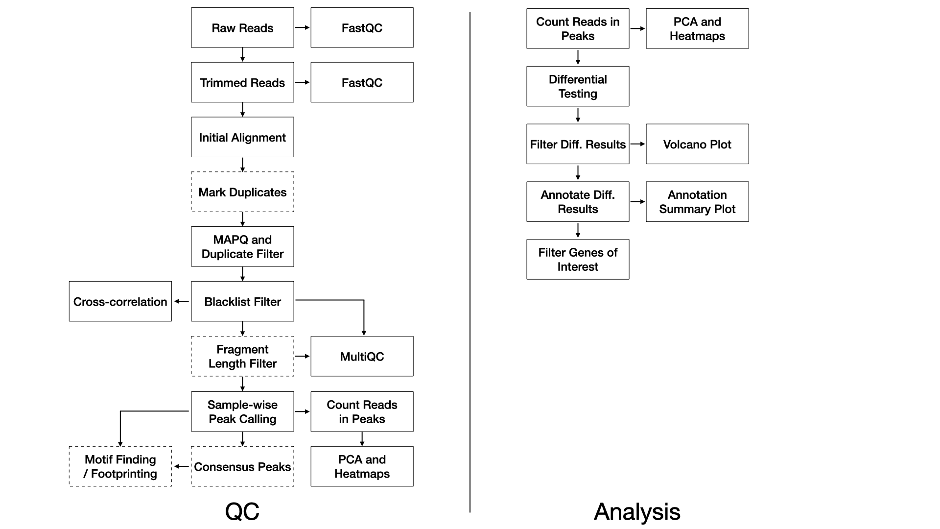
We use FastQC (FastQC) (v0.11.8) to assess the overall quality of each sequenced sample.
We use TrimGalore (TrimGalore) (v0.4.5) and cutadapt
(Martin) (v1.15) with the following
parameters:
--nextera -e 0.1 --stringency 6 --length 20 --nextseq 20.
We align trimmed reads to the reference genome with Bowtie2 (Langmead and Salzberg, 2012) (v2.3.4.1) using
default parameters with the exception of the following flags:
-X 2000.
Duplicate reads may be are marked with Picard (Picard) (v2.20.2).
Alignments are filtered with samtools (Li
et al., 2009) (v1.2) using the flags:
-q 10 -F 1024.
Alignments completely overlapping blacklisted regions (ENCODE Blacklist Regions) are removed with bedtools (Quinlan and Hall, 2010) (v2.28.0).
Sample-wise peaks are called with macs2 (Zhang
et al., 2008) (v2.1.2) with flags:
--format BAMPE --gsize mm --qvalue 0.05.
Optionally, consensus peaks for replicates are determined by mutual intersection of sample-wise peaks with bedops –intersect. Consensus peaks are then annotated with annotatr (Cavalcante and Sartor, 2017).
Optionally, motifs for consensus peaks are found with HOMER (Heinz et al., 2010) (v4.11.1).
Peaks over all samples are merged with bedops (Neph et al., 2012) (v2.4.36) for the purpose of principal component analysis and unsupervised clustering to assess the similarity of samples. Read cross-correlations within samples are plotted using phantompeakqualtools (Landt et al., 2012). MultiQC (Ewels et al., 2016) (v1.7) generates a report combining FastQC, trimming, alignment, and duplicate calling over all the samples. The software DeepTools is used to calculate coverage and IP efficiency plots (Ramírez et al., 2016) (v3.3.0).
Differential Testing
We use the edgeR R Bioconductor package (McCarthy et al., 2012) to identify regions of differential binding. For each sample, the number of reads in the merged peaks is counted for each sample, and a library size normalization factor is determined. With no replicates, we manually tune the BCV (biological coefficient of variance) parameter. We then fit each model using the glmFit function, and test each contrast with a likelihood ratio test. With replicates, the common, trended, and tagwise negative binomial dispersions are calculated. We then fit each model using the glmQLFit function, and test each contrast with an empirical Bayes quasi-likelihood F-test. The differential peaks are then annotated to genic and CpG island annotations using the annotatr R Bioconductor package (Cavalcante and Sartor, 2017).