Getting Started with Seurat
UM Bioinformatics Core Workshop Team
2025-10-16
Introduction
|
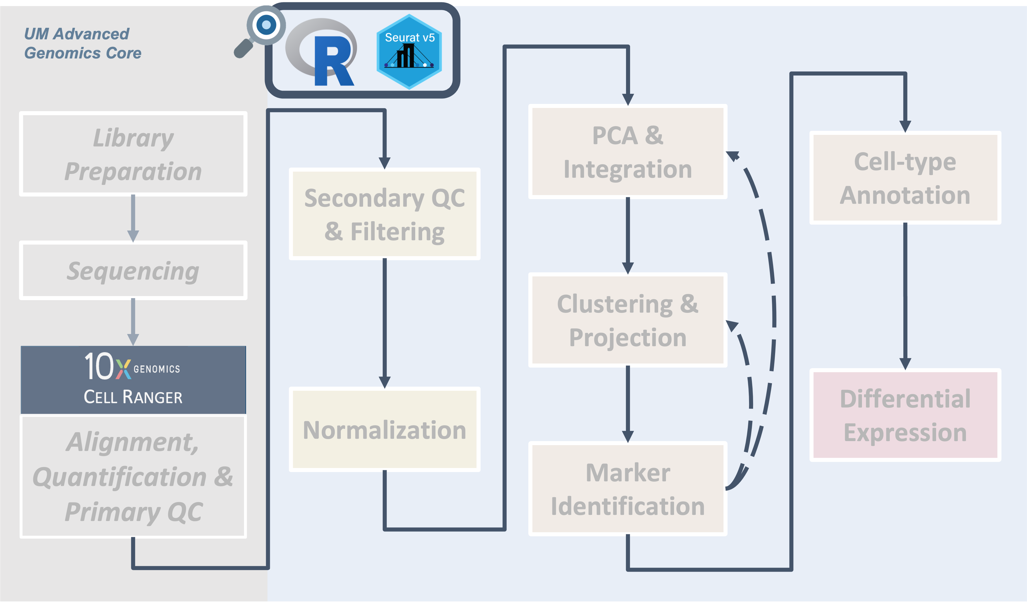
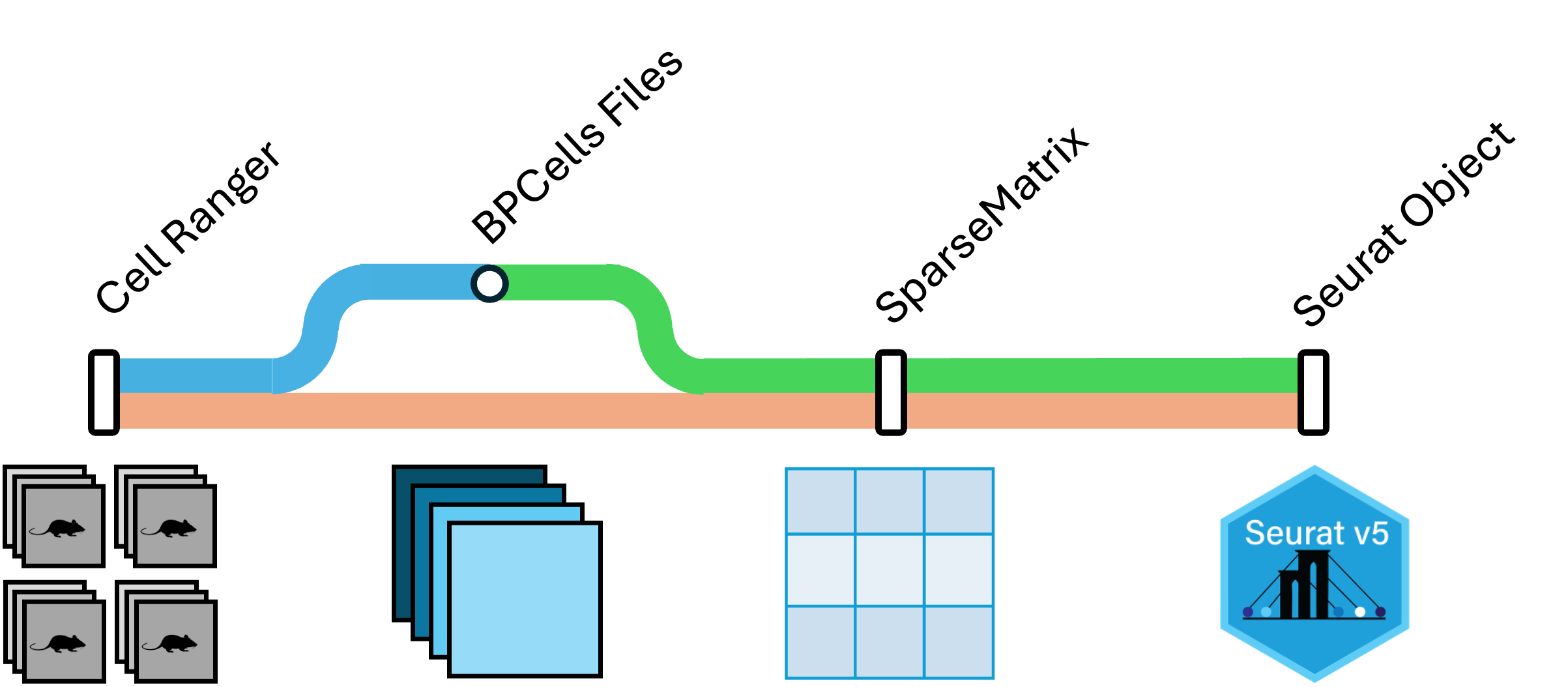
| Cell Ranger outputs can be read into R via the triple of files directly, or via a memory saving route with the BPCells package. We provide code for both routes in this section. |
Objectives
- Orient on RStudio.
- Create an RStudio project for analysis.
- Create directory structure for analysis.
- Learn how to read Cell Ranger data into Seurat.
- Introduce the Seurat object, and how to access parts of it.
Server login
Let’s log in to the workshop server: http://bfx-workshop02.med.umich.edu
The login page for the server looks like:
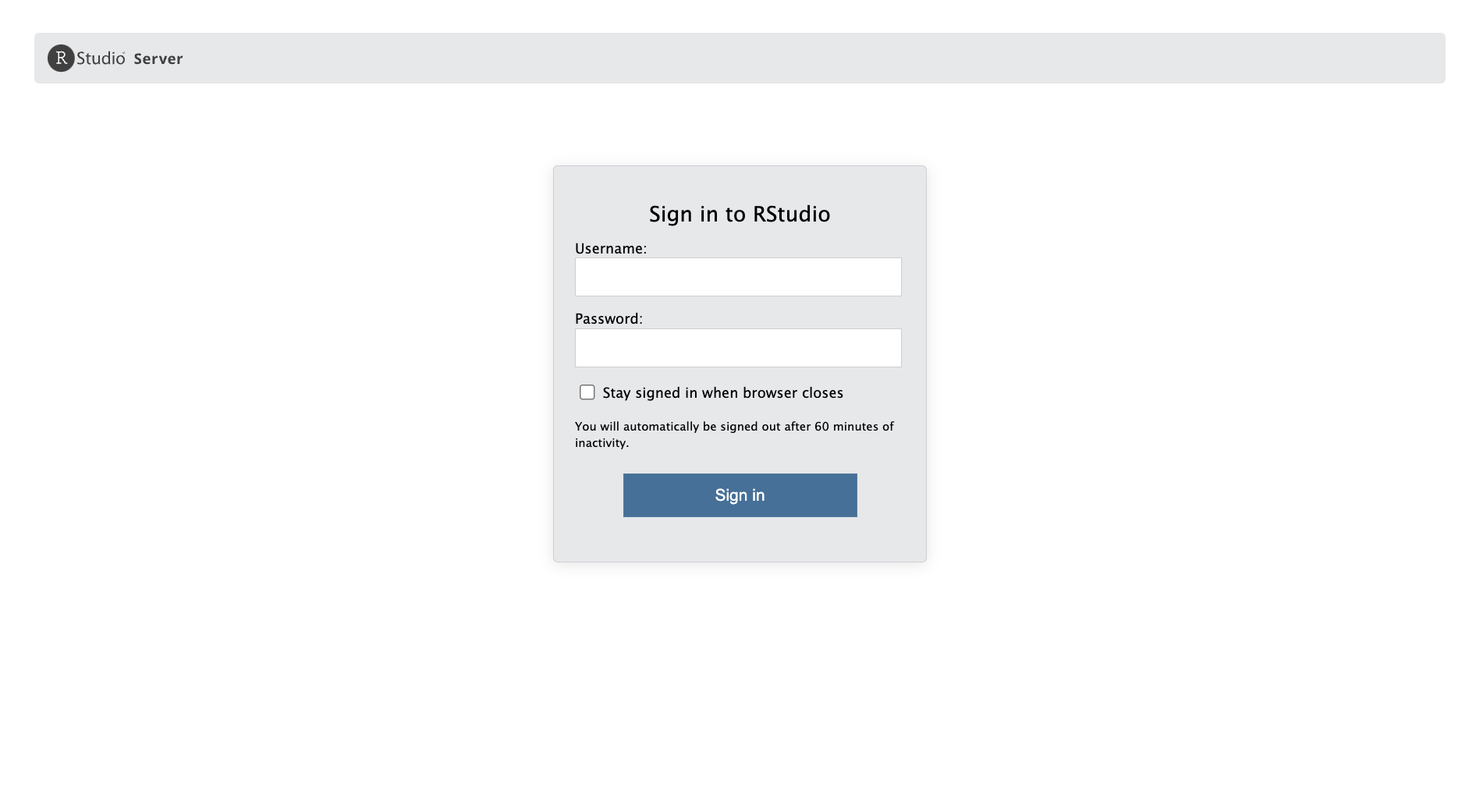
Enter your user credentials and click Sign In. The RStudio interface should load and look like:
Checkpoint
Create a project
We will create an RStudio Project to easily keep track of our working directory. See the Projects section of R for Data Science for a more in-depth description of what a project is and how it’s helpful.
To create a Project, click File then New
Project…. In the New Project Wizard window that opens, select
Existing Directory, then Browse…. In the Choose
Directory window, select the ISC_R folder by clicking it
once, and then click the Choose button. Finally, click
Create Project.
Once we do this, RStudio will restart and the Files pane (lower
right) should put us in the ~/ISC_R folder where there is
an inputs/ folder and an ISC_R.Rproj file.
Checkpoint
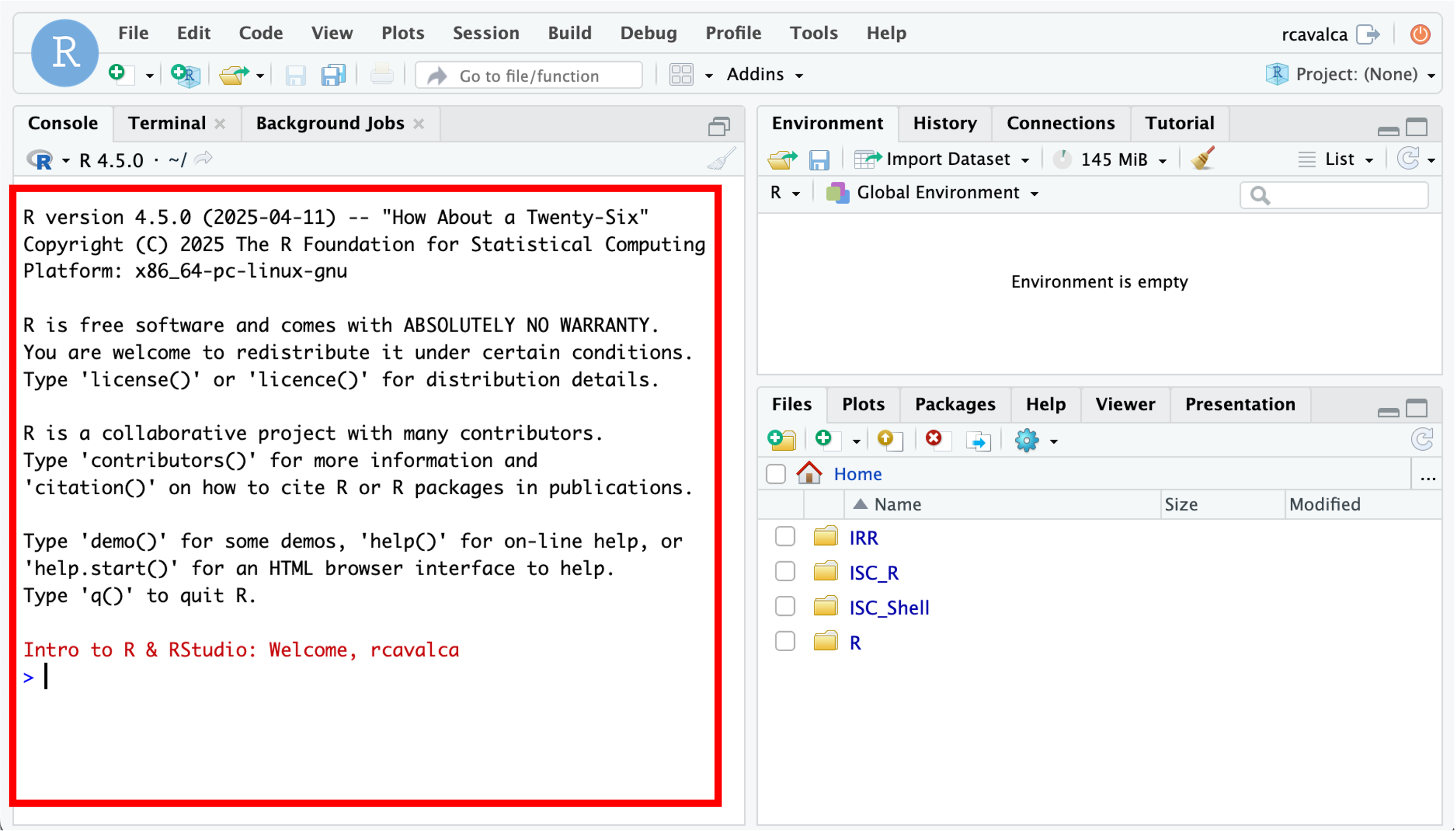
The RStudio interface
RStudio is an integrated development environment where you can write, execute, and see the results of your code. The interface is arranged in different panes:
- The Console pane along the left where you can enter commands and execute them.
- The Environment pane in the upper right shows any variables you have created, along with their values.
- The pane in the lower right has a few functions:
- The Files tab let’s you navigate the file system.
- The Plots tab displays any plots from code run in the Console.
- The Help tab displays the documentation of functions.
Commands in the Console
Working directly in the console is working directly with R. Commands can be entered and run with the Enter key:
> 2+2
[1] 4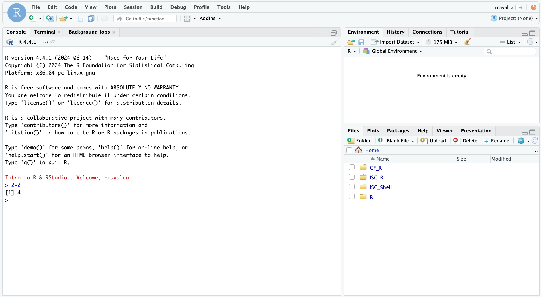
Checkpoint
Commands in a Script
Instead of entering commands directly into the Console, we’ll record them in and run them from a script. Some benefits to using a script rather than using the Console pane:
- Scripts record the steps taken to analyze the data.
- Scripts can be re-run, allowing for reproducibility.
- Scripts are can be shared.
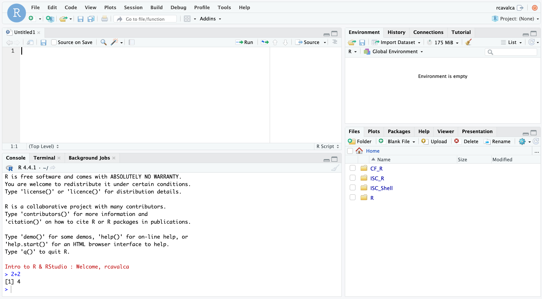
We’ll create a script file by clicking on the icon in the upper-left of the interface (a blank piece of paper with a + sign), and selecting R Script.
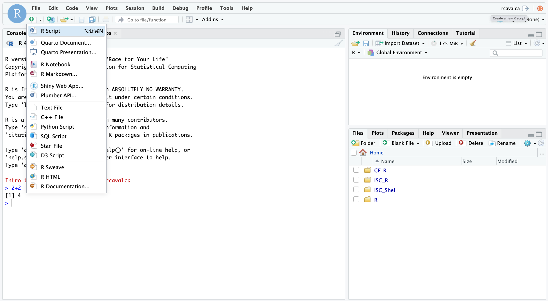
The new pane that opens is the Source pane, and you can think of it as a text editor:
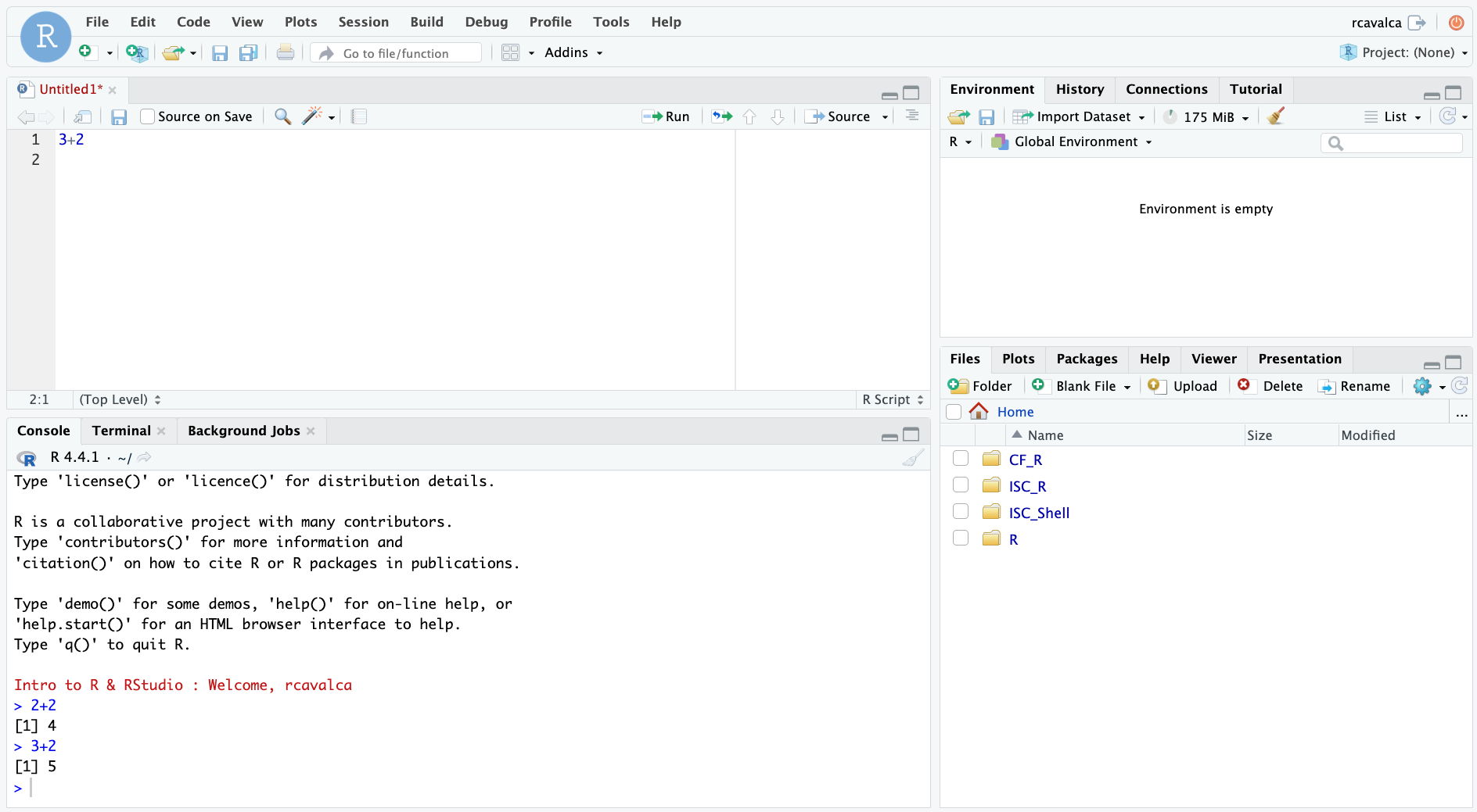
Code entered in a script file must explicitly be sent to the Console for execution with the Ctrl + Enter command. Enter the following command into the script file and execute it with Ctrl + Enter:
3+2Looking in the Console we see the executed line and its result. Note that pressing Enter in the script creates a new line and does not execute the code as in the Console.
Console vs Script
The key differences between the Console and Script panes in RStudio:
| Console | Script |
|---|---|
| Reset across sessions | Preserved acros sessions |
| Run with Enter | Run with Ctrl + Enter |
| Inconvenient to share | Convenient to share |
Configuring RStudio
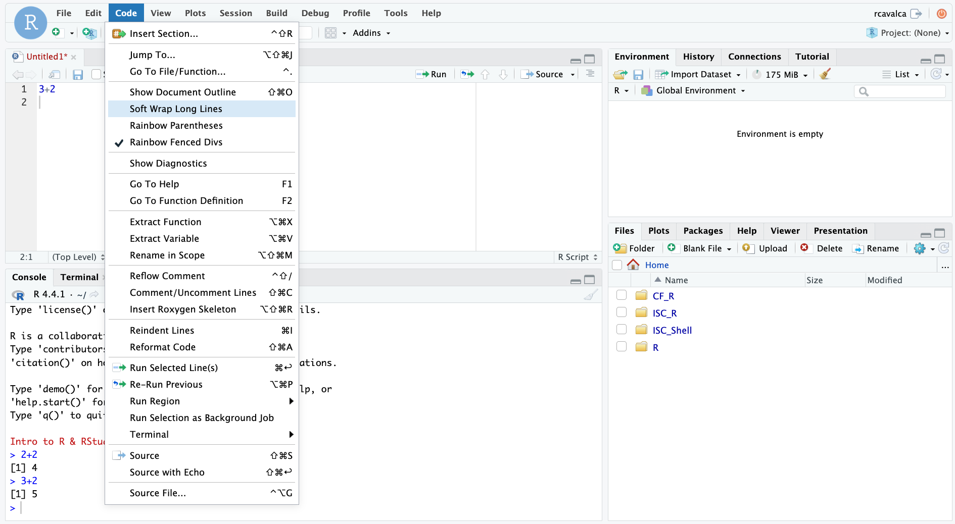
All of the panes in RStudio have configuration options. For example, you can minimize/maximize a pane or resize panes by dragging the borders. The most important customization options for pane layout are in the View menu. Other options such as font sizes, colors/themes, and more are in the Tools menu under Global Options.
We can enable soft-wrapping of code by selecting Code and then Soft Wrap Long Lines.
Workshop flow
To accommodate different learning styles and to keep us moving along, we’ll provide code in three different ways, and you can get that code into RStudio in corresponding ways:
| Source of Code | Execution of Code |
|---|---|
| Zoom screen share | Type the code yourself. |
| Slack | Copy and paste into RStudio. |
| Website | Copy with code block button and paste into RStudio. |
Questions?
Directory structure
Before we begin, the folder structure of a project organizes all the relevant files. Typically we make directories for the following types of files:
- Raw data, called
data,input, etc, - Results, often
resultsoroutputwith subfolders fortables,figures, andrdata, and - Scripts, often
scripts.
We’ve already provided the raw data in the data/ folder,
and it’s generally a good idea to keep raw data in its own folder.
Let’s create some folders for our analysis scripts and results thereof.
# -------------------------------------------------------------------------
# Create directory structure

dir.create('scripts', recursive = TRUE, showWarnings = FALSE)
dir.create('results/figures', recursive = TRUE, showWarnings = FALSE)
dir.create('results/tables', recursive = TRUE, showWarnings = FALSE)
dir.create('results/rdata', recursive = TRUE, showWarnings = FALSE)
Saving scripts
Let’s save our currently open script by clicking File and
then Save. Double click the scripts/ folder and
enter the file name ISC_day1.R.
Checkpoint
Loading libraries
We begin our analysis script by loading the libraries we expect to
use. It’s generally good practice to include all library()
calls at the top of a script for visibility.
# -------------------------------------------------------------------------
# Load libraries
library(Seurat)
library(BPCells)
library(tidyverse)

options(future.globals.maxSize = 1e9)
The libraries that we are loading are:
- The
Seuratlibrary, developed by the Satija lab, which will provide the essential functions used in our single-cell analysis. The Seurat documentation is extensive and indispensible. - The
BPCellslibrary, developed by Benjamin Parks, is a recent package with the primary goal of efficiently storing single-cell data to reduce its memory footprint. The BPCells documentation includes many useful tutorials. - The
tidyverselibrary, developed by Posit, is an essential package for data manipulation and plotting. The tidyverse documentation is essential for getting a handle on the array of functions in the many packages contained therein.
Read in data
The inputs/10x_cellranger_filtered_triples/ folder is
closer to what AGC would generate with Cell Ranger, where each sample
has a folder, and within that folder there are three files:
barcodes.tsv.gzfeatures.tsv.gzmatrix.mtx.gz
Note, these files are filtered matrices, AGC will touch on filtered and unfiltered Cell Ranger outputs.
Read10X
The Read10X() function will read in the triples
organized within sample folders:
# -------------------------------------------------------------------------
# To load data from 10X Cell Ranger

# Collect the input directories
#   Each sample dir contains barcodes.tsv.gz, features.tsv.gz, matrix.mtx.gz.
#   Naming the sample_dirs vector makes Seurat name the
#     samples in the corresponding manner, which is nice for us.
sample_dirs = list(
  HODay0replicate1  = "~/ISC_R/inputs/10x_cellranger_filtered_triples/count_run_HODay0replicate1",
  HODay0replicate2  = "~/ISC_R/inputs/10x_cellranger_filtered_triples/count_run_HODay0replicate2",
  HODay0replicate3  = "~/ISC_R/inputs/10x_cellranger_filtered_triples/count_run_HODay0replicate3",
  HODay0replicate4  = "~/ISC_R/inputs/10x_cellranger_filtered_triples/count_run_HODay0replicate4",
  HODay7replicate1  = "~/ISC_R/inputs/10x_cellranger_filtered_triples/count_run_HODay7replicate1",
  HODay7replicate2  = "~/ISC_R/inputs/10x_cellranger_filtered_triples/count_run_HODay7replicate2",
  HODay7replicate3  = "~/ISC_R/inputs/10x_cellranger_filtered_triples/count_run_HODay7replicate3",
  HODay7replicate4  = "~/ISC_R/inputs/10x_cellranger_filtered_triples/count_run_HODay7replicate4",
  HODay21replicate1 = "~/ISC_R/inputs/10x_cellranger_filtered_triples/count_run_HODay21replicate1",
  HODay21replicate2 = "~/ISC_R/inputs/10x_cellranger_filtered_triples/count_run_HODay21replicate2",
  HODay21replicate3 = "~/ISC_R/inputs/10x_cellranger_filtered_triples/count_run_HODay21replicate3",
  HODay21replicate4 = "~/ISC_R/inputs/10x_cellranger_filtered_triples/count_run_HODay21replicate4")

# Create the expression matrix from sample dirs
#   Read10X needs a *vector* instead of a *list*, so we use *unlist* to convert
geo_mat = Read10X(data.dir = unlist(sample_dirs))
Write BPCells
We could create a Seurat object with
CreateSeuratObject(counts = geo_mat), but we will first
output geo_mat using the BPCells package to save
memory:
# -------------------------------------------------------------------------
# Build BPCells input dir
# To use BPCells (to save some memory), you can transform
# the expression matrix data structure above into BPCells files.
# BPCells uses these files for processing, but you typically never look at
# their contents directly
write_matrix_dir(mat = geo_mat, dir = '~/ISC_R/bpcells', overwrite = TRUE)
Warning: Matrix compression performs poorly with non-integers.
• Consider calling convert_matrix_type if a compressed integer matrix is intended.
This message is displayed once every 8 hours.32285 x 35269 IterableMatrix object with class MatrixDir
Row names: Xkr4, Gm1992 ... AC149090.1
Col names: HODay0replicate1_AAACCTGAGAGAACAG-1, HODay0replicate1_AAACCTGGTCATGCAT-1 ... HODay21replicate4_TTTGTCACAGGGAGAG-1
Data type: double
Storage order: column major
Queued Operations:
1. Load compressed matrix from directory /home/workshop/damki/ISC_R/bpcells# -------------------------------------------------------------------------
# Cleanup
# Since we'll now be reading in from BPCells files, we will remove geo_mat
# from the environment and then prompt RStudio to run a "garbage collection"
# to free up unused memory
rm(geo_mat)
gc() used (Mb) gc trigger (Mb) max used (Mb)
Ncells 6342912 338.8 11330051 605.1 8186707 437.3
Vcells 11857303 90.5 564817080 4309.3 673134891 5135.7Read BPCells
Let’s read the BPCells files in, and note that the
geo_mat object takes up less memory than when we created it
with Read10X():
# -------------------------------------------------------------------------
# Create expression matrix and Seurat object from BPCells files
geo_mat = open_matrix_dir(dir = '~/ISC_R/bpcells')
Create a Seurat object
The expression matrix is the precursor to creating the
Seurat object upon which all our analysis will be done. To
create the Seurat object:
# -------------------------------------------------------------------------
# Create seurat object
geo_so = CreateSeuratObject(counts = geo_mat, min.cells = 1, min.features = 50)
geo_so
An object of class Seurat
26489 features across 35216 samples within 1 assay
Active assay: RNA (26489 features, 0 variable features)
1 layer present: countsWe have specified some parameters to remove genes and cells which do not contain very much information. Specifically a gene is removed if it is expressed in 1 or fewer cells, and a cell is removed if it contains reads for 50 or fewer genes. In the context of this workshop, this helps us minimize memory usage.
molecule_info.h5 as an alternative input to Seurat
H5 (aka HDF5) is an alternative file format
Some programs (like Seurat) need only the barcodes, features, and matrix (counts) and those data are conveniently provided as three separate files for each sample. Other programs (like Cell Ranger) need to store more information (e.g. probe info about certain library preps or the chip or channel that cell ran on). Instead of adding more files to complement the three base files above, 10x provides a single binary file, molecule_info.h5, which contains all information for all molecules. (Strictly only the molecules with valid barcode/UMI assigned to a gene.)
- molecule_info.h5 is a single file, but with really acts like basket of related structures (think tables) for a single sample.
- The “.h5” extension stands for HDF5, a broadly adopted, platform agnostic, scalable, high-performance file format for storing complex data.
- You can view the data within the .h5 file with special tools like HDF5View or h5dump. Here is an excerpt of the structures inside that file:
molecule_info.h5
    ├─ barcodes [HDF5 group]
    ├─ count
    ├─ features [HDF5 group]
    ├─ gem_group
    ├─ library_info
    ├─ metrics_json
    ├─ probes [HDF5 group]
    ├─ ...
    └─ umi
You can see the first structures above are barcodes, features, and counts. So if you have the hdf5 libraries installed, you can use the .h5 as input to Seurat like so:
# ==========================================================================
### DO NOT RUN ###
# To load data from raw .h5 file
### DO NOT RUN ###

HODay0replicate1 = "~/ISC_Shell/cellranger_outputs/count_run_HODay0replicate1/outs/molecule_info.h5"
get_mat = Read10X_h5(filename = HODay0replicate1)
geo_so = CreateSeuratObject(counts = geo_mat, min.cells = 1, min.features = 50)
If you want to load multiple samples from .h5 files, see the function Read10X_h5_Multi_Directory in the scCustomize R library.
FYI
- Be aware, using HDF5 files from R support requires the hdf5 library which entails a few more steps to install than a typical library. Brew a nice cup of (decaf) tea and review how to install hdf5.
- See the Seurat function Read10X.
- See BPCells docs for details on loading from h5 to a BPCells directory.
- 10x Genomics details the full contents of molecule_info.h5.
- Checkout the HDF5 reference docs for more information about the HDF5 format.
Structure of a Seurat object
The Seurat object is a complex data type, so let’s get a
birds eye view with an image from this
tutorial on single-cell analysis.

The three main “slots” in the object are:
- The assays slot stores the expression data as
Assayobjects. - The meta.data slot which stores cell-level information, including technical and phenotypic data.
- The reductions slot stores the results of dimension
reduction applied to the
assays.
There are other slots which store information that becomes relevant as we progress through the analysis. We will highlight the other slots as they come up.
After reading the data in and creating the Seurat object above, we can imagine the following schematic representing our object:
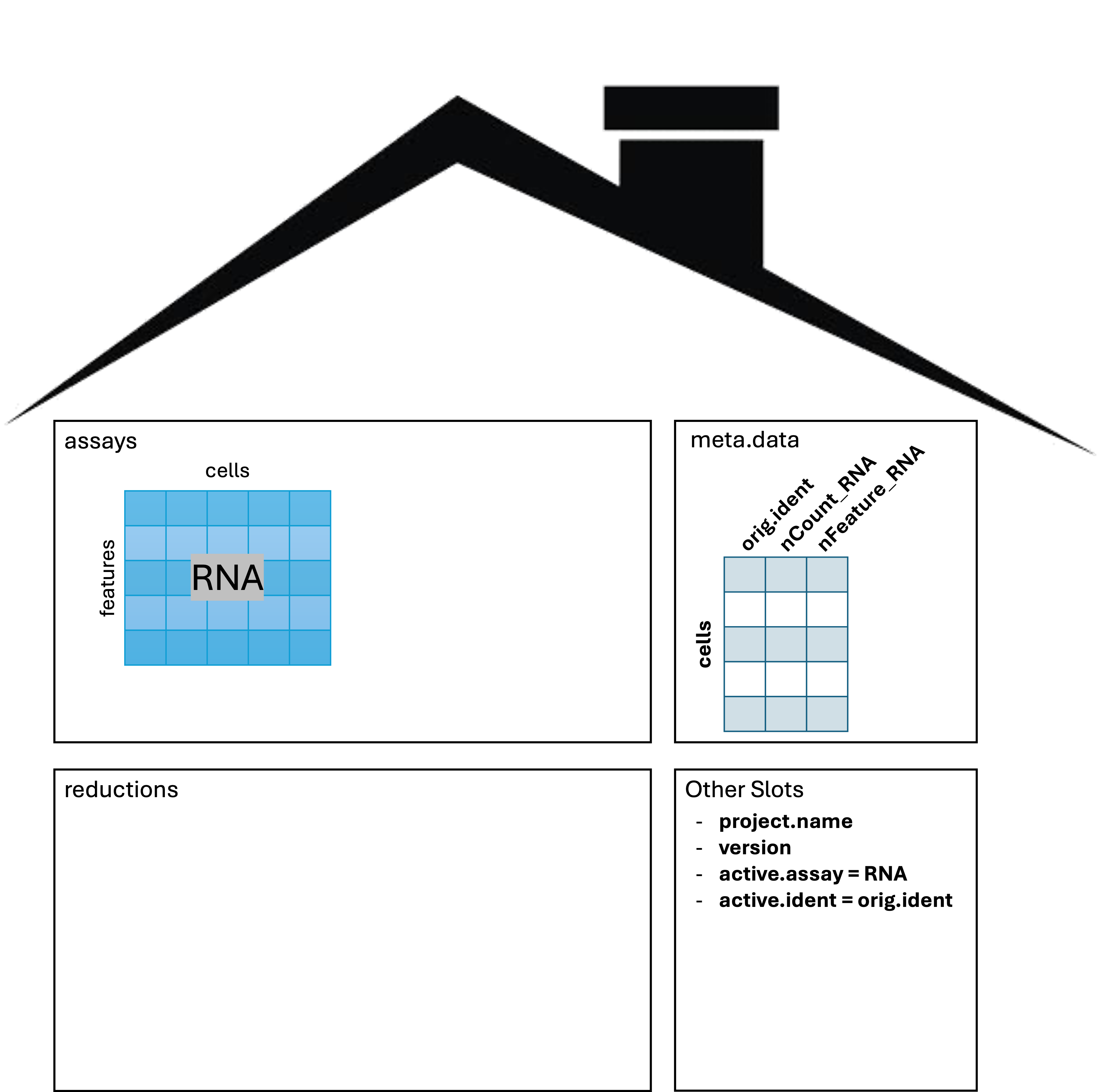
Note the RNA assay contains a count layer consisting of
a raw count matrix where the rows are genes (features, more
generically), and the columns are all cells across all samples. Note
also the presence of a meta.data table giving information
about each cell. We’ll pay close attention to this as we proceed. The
other slots include information about the active.assay and
active.ident which tell Seurat which expression data to use
and how the cells are to be identified.
Accessing parts of the object
The only slot of the Seurat object that we’ll typically
access or modify by hand–that is, without a function from the
Seurat package–is the meta.data object. In R,
slots are accessed with the @ symbol, as in:
# -------------------------------------------------------------------------
# Examine Seurat object
head(geo_so@meta.data)
orig.ident nCount_RNA
HODay0replicate1_AAACCTGAGAGAACAG-1 HODay0replicate1 10234
HODay0replicate1_AAACCTGGTCATGCAT-1 HODay0replicate1 3158
HODay0replicate1_AAACCTGTCAGAGCTT-1 HODay0replicate1 13464
HODay0replicate1_AAACGGGAGAGACTTA-1 HODay0replicate1 577
HODay0replicate1_AAACGGGAGGCCCGTT-1 HODay0replicate1 1189
HODay0replicate1_AAACGGGCAACTGGCC-1 HODay0replicate1 7726
nFeature_RNA
HODay0replicate1_AAACCTGAGAGAACAG-1 3226
HODay0replicate1_AAACCTGGTCATGCAT-1 1499
HODay0replicate1_AAACCTGTCAGAGCTT-1 4102
HODay0replicate1_AAACGGGAGAGACTTA-1 346
HODay0replicate1_AAACGGGAGGCCCGTT-1 629
HODay0replicate1_AAACGGGCAACTGGCC-1 2602Here, each row is a cell, and each column is information about that
cell. The rows of the table are named according to the uniquely
identifiable name for the cell. In this case, the day and replicate, as
well as the barcode for that cell. As we continue the workshop, we will
check in on the meta.data slot and observe changes we want
to make, and that other functions will make. We’ll also observe the
other assays and layers and note their changes.
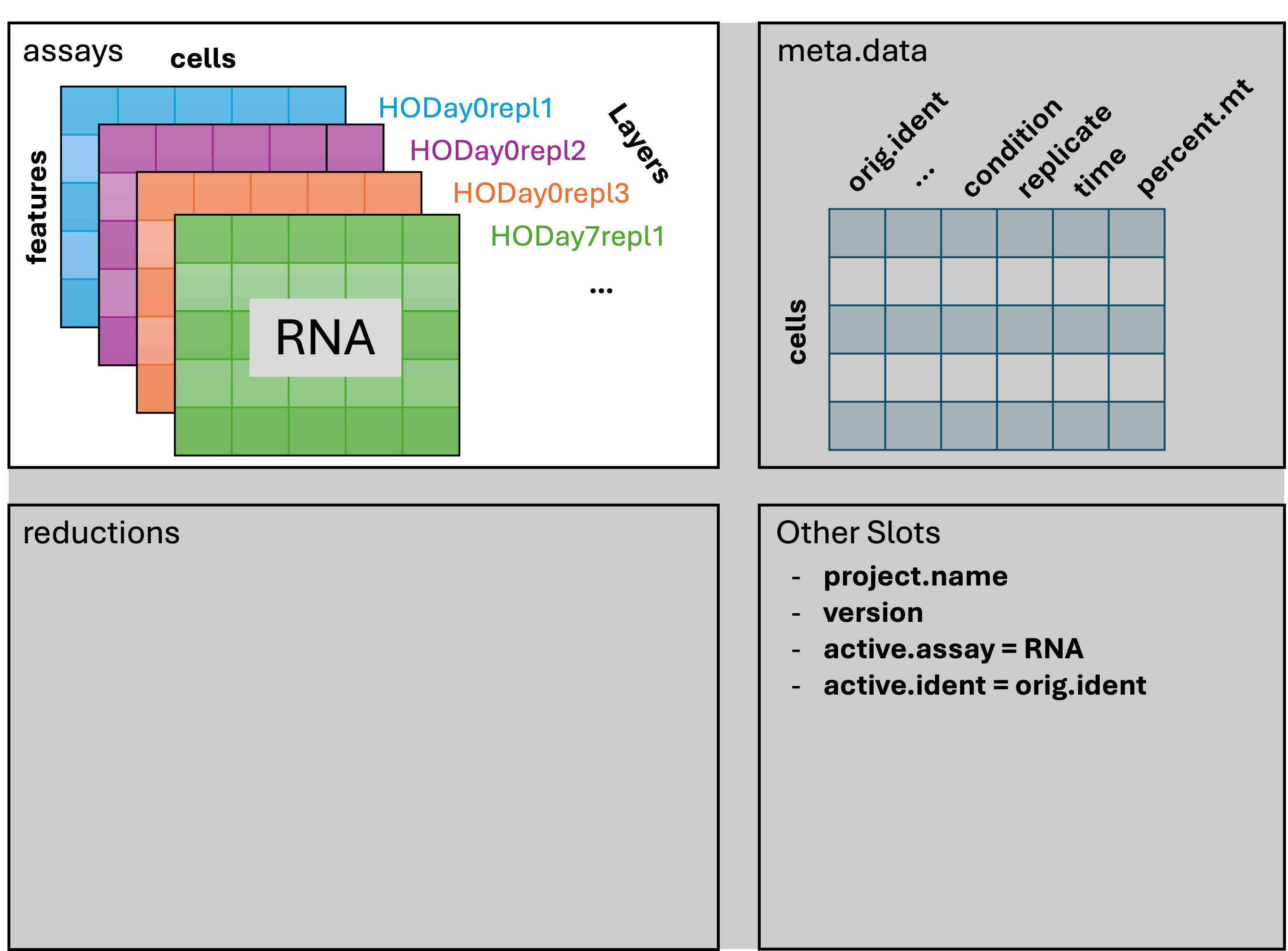
Splitting samples
The assays in a Seurat v5 object can store data in layers; a layer is the data for a single sample. Initially there is only a single layer, can separate the sample-wise data into layers like so:
# -------------------------------------------------------------------------
# Separate sample data into layers
geo_so[['RNA']] = split(geo_so[['RNA']], f = geo_so$orig.ident)
geo_so
An object of class Seurat
26489 features across 35216 samples within 1 assay
Active assay: RNA (26489 features, 0 variable features)
12 layers present: counts.HODay0replicate1, counts.HODay0replicate2, counts.HODay0replicate3, counts.HODay0replicate4, counts.HODay7replicate1, counts.HODay7replicate2, counts.HODay7replicate3, counts.HODay7replicate4, counts.HODay21replicate1, counts.HODay21replicate2, counts.HODay21replicate3, counts.HODay21replicate4We see the 12 layers containing the count data for each of the samples. Our Seurat object now looks like this:
Save our progress
Let’s Save our progress as an RDS file with saveRDS();
this allows us to have a copy of the object that we can read back into
our session with the readRDS() commmand. Periodically we
will be saving our Seurat object so that we can have a version of it at
different steps of the analysis. These will also help us get untangled
if we get into an odd state.
# -------------------------------------------------------------------------
# Save the Seurat object
saveRDS(geo_so, file = 'results/rdata/geo_so_unfiltered.rds')
Now that the state of our analysis is saved on disk, we’ll demonstrate how to power down the RStudio session, restart the session, and re-load the data we just saved.
- To power down the session, click the orange power button in the upper right corner of the RStudio window. Note: There is no confirmation dialogue, the session will simply end.
- Click the “Start New Session” button to restart the RStudio session.
- Re-load the
geo_soobject with:
# -------------------------------------------------------------------------
# Load libraries
library(Seurat)
library(BPCells)
library(tidyverse)
options(future.globals.maxSize = 1e9)

# -------------------------------------------------------------------------
# Load the Seurat object
geo_so = readRDS('results/rdata/geo_so_unfiltered.rds')
Pro-tip: RStudio, Seurat, and Memory
R and RStudio are designed to grab computer memory (RAM) when necessary and release that memory when it’s no longer needed. R does this with a fancy computer science technique called garbage collection.
The R garbage collector is very good for small objects and simple analyses, but complex single-cell analysis can overwhelm it. So don’t rely on R/RStudio’s built in garbage collection and session management for single-cell analysis. Instead, do the following:
- Save intermediate versions of the Seurat object as you go along
using
saveRDS(). This gives you “savepoints” so if you need to backtrack, you don’t have to go back to the beginning. - Save ggplots into image files as you go along. Periodically clear
ggplot objects from the R environment.
- At the end of each day, wherever you are in the analysis, explicitly
save the Seurat object and “power down” your session.
- The next day, you can load the Seruat object using readRDS().
This simple pattern will make your code more reproducible and your RStudio session more reliable.
Summary
|
|
| Cell Ranger outputs can be read into R via the triple of files directly, or via a memory saving route with the BPCells package. We provide code for both routes in this section. |
In this section we:
- Created an RStudio project for analysis.
- Created the directory structure for analysis.
- Learned how to read 10X data into Seurat.
- Introduced the Seurat object, and how to access parts of it.
- Learned some tips on managing memory.
- Learned to save our work and also to stop and restart the RStudio session.
References:
- Seurat documentation
- BPCells documentation
- tidyverse documentation
- How R uses memory
- Memory monitoring in RStudio
Acknowledgements These materials have been adapted and extended from materials listed above. These are open access materials distributed under the terms of the Creative Commons Attribution license (CC BY 4.0), which permits unrestricted use, distribution, and reproduction in any medium, provided the original author and source are credited.
| Previous lesson | Top of this lesson | Next lesson |
|---|