Normalization
UM Bioinformatics Core Workshop Team
2025-10-16
Introduction
|
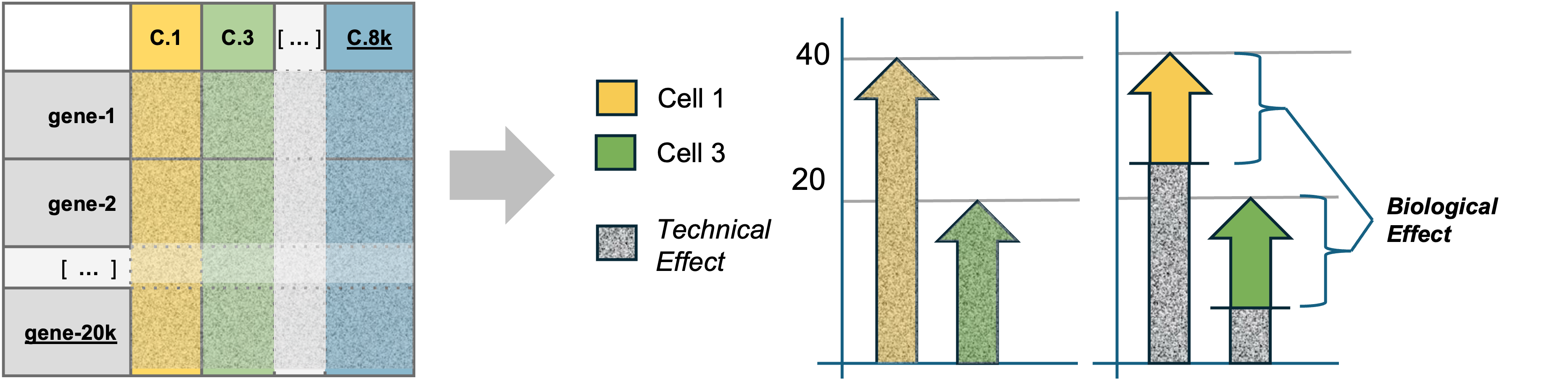
| The counts in the feature barcode matrix are a blend of technical and biological effects. Technical effects can distort or mask the biological effects of interest, confounding downstream analyses. Seurat can model the technical effects based on overall patterns in expression across all cells. Once these technical effects are minimized, the remaining signal is primarily due to biological variance. |
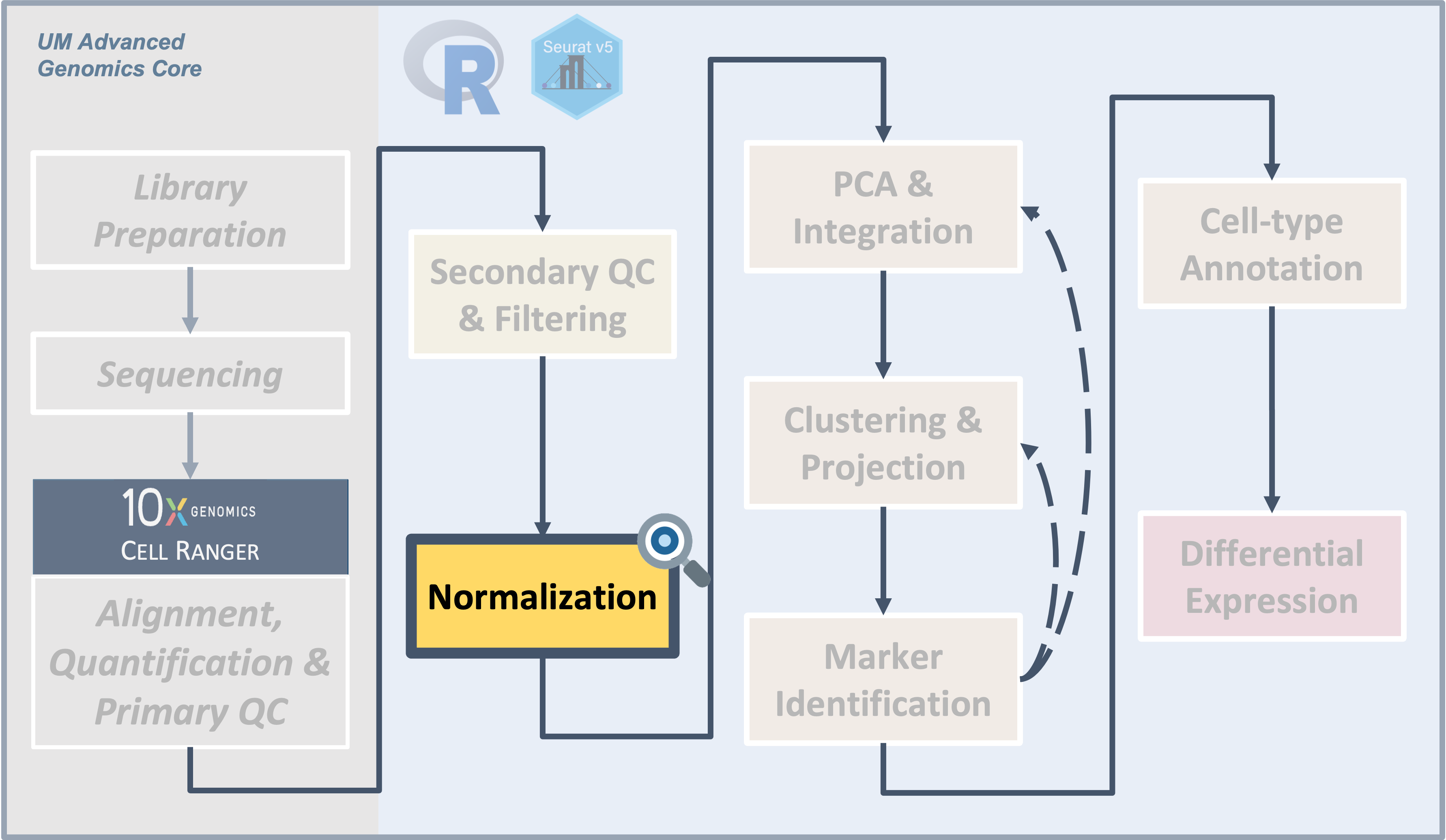
After removing low-quality cells from the data, the next task is the
normalization and variance stabilization of the counts to prepare for
downstream analysis including integrating between samples and
clustering.
Objectives
- Understand why normalization is needed.
- Describe the essence of the
SCTransform()method. - Understand normalization options.
- Normalize the counts with
SCTransform().
Normalization
Motivation
Variation in scRNA-seq data comes from biological sources:
- Differences in cell type or state
- Differences in response to treatment
And from technical sources:
- Fluctuations in cellular RNA content
- Efficiency in lysis and reverse transcription
- Stochastic sampling during sequencing
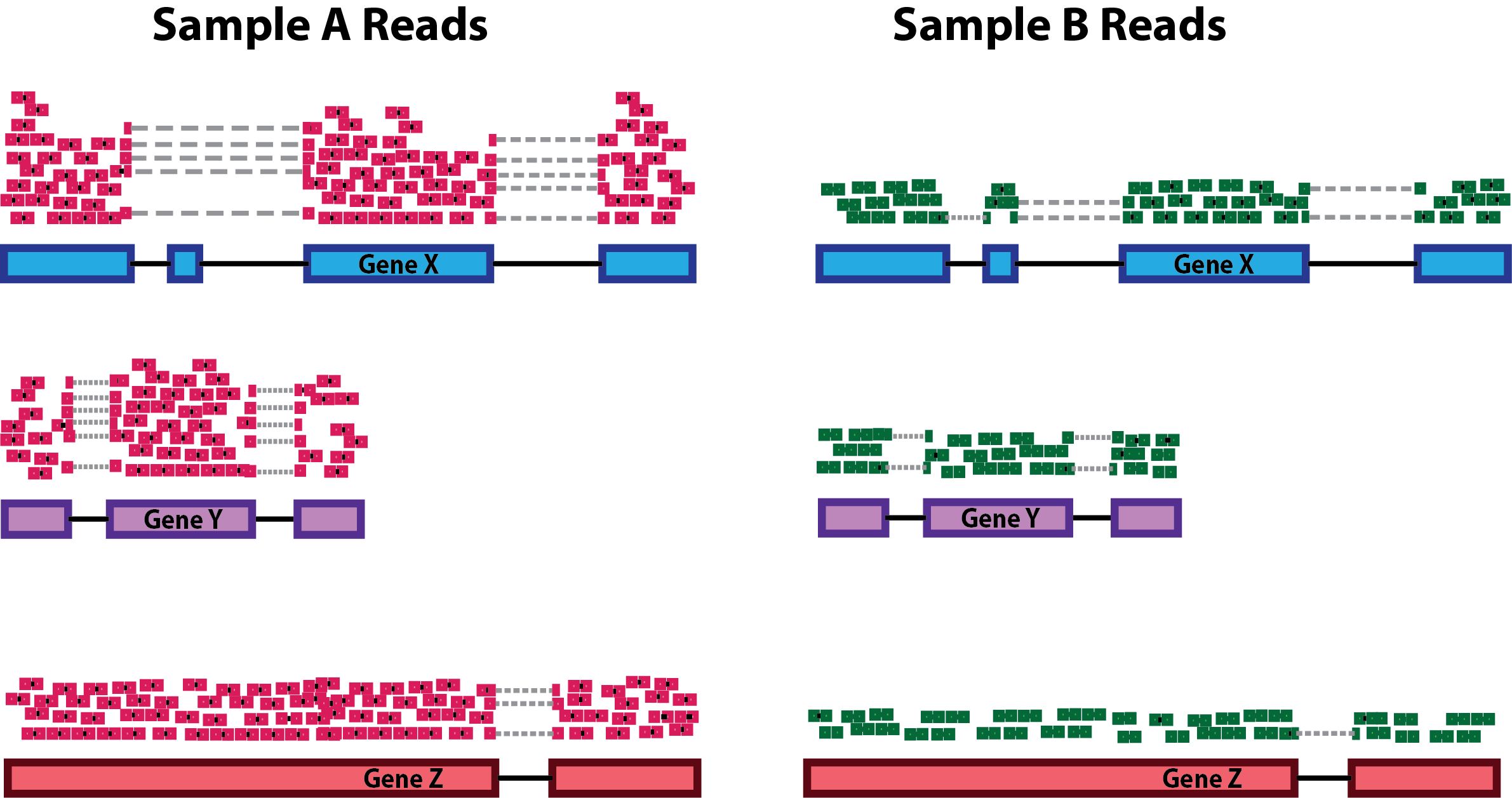
A key driver of technical variation is cellular sequencing depth (that is, the number of UMIs sequenced per cell). In the figure below, Sample A (left, red reads) is more deeply sequenced than Sample B (right, green reads). In a test for differential expression, we want to account for the difference in sequencing depth to avoid erroneously calling a gene differentially expressed.
Here is our current Seurat object
The command SCTransform() normalizes the data. It takes
a long time to run, so we’ll start the command and while it executes, we
can consider what it’s doing.
# =========================================================================
# Normalization
# =========================================================================

# -------------------------------------------------------------------------
# Normalize the data with SCTransform
geo_so = SCTransform(geo_so)

# See the new SC
Assays(geo_so)
[1] "RNA" "SCT"geo_soAn object of class Seurat
46957 features across 31559 samples within 2 assays
Active assay: SCT (20468 features, 3000 variable features)
3 layers present: counts, data, scale.data
1 other assay present: RNANormalization explained
To get the idea of what SCTransform() is doing, we’ll
consider a simplified example.
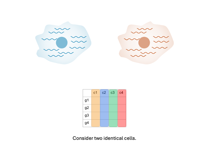
Consider two cells that are identical in terms of their type, expression, etc. Imagine that we put them through the microfluidic device and then sequenced the RNA content.
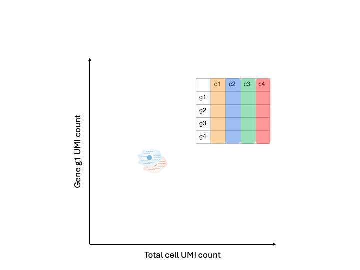
If we were to plot the total cell UMI count against a particular gene UMI count, in an ideal world, the points should be directly on top of each other because the cells had identical expression and everything done to measure that expression went perfectly.
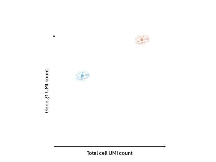
However, we don’t live in a perfect world. We will likely observe the cells have different total cell UMI counts as well as different gene UMI counts. This difference, given that the cells were identical, can be attributed to technical factors. For example, efficiency in lysis or in reverse transcription, or the stoachastic sampling that occurs during sequencing.
It is these technical factors that normalization seeks to correct for, getting us back to the “true” expression state.
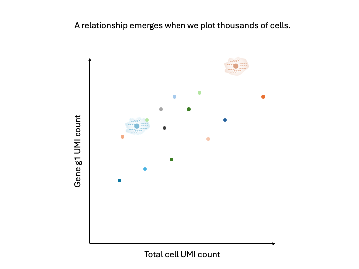
Imagine doing this for thousands of cells. We would get a point cloud like the above. Importantly, that point cloud has structure. There is a relationship between the total cell UMI count and the gene UMI count for each gene.
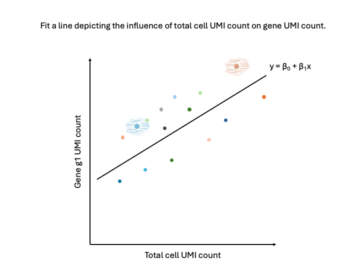
We could fit a line through the point cloud, where we estimate the intercept, the slope, and the error.
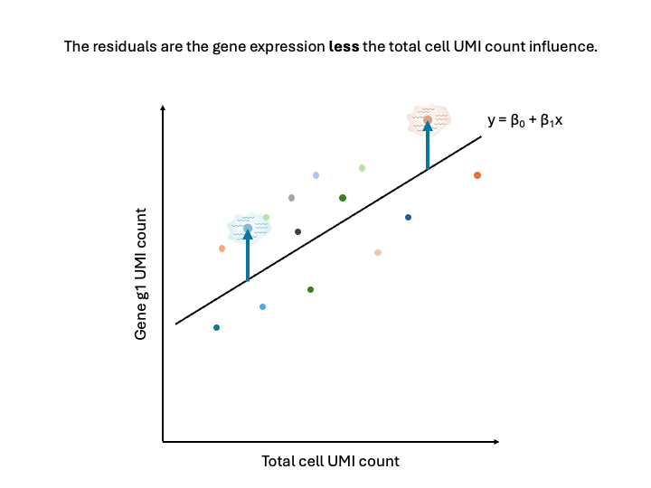
The residuals, or the distance from the point to the line, represents the expression of the gene less the total cell UMI count influence.
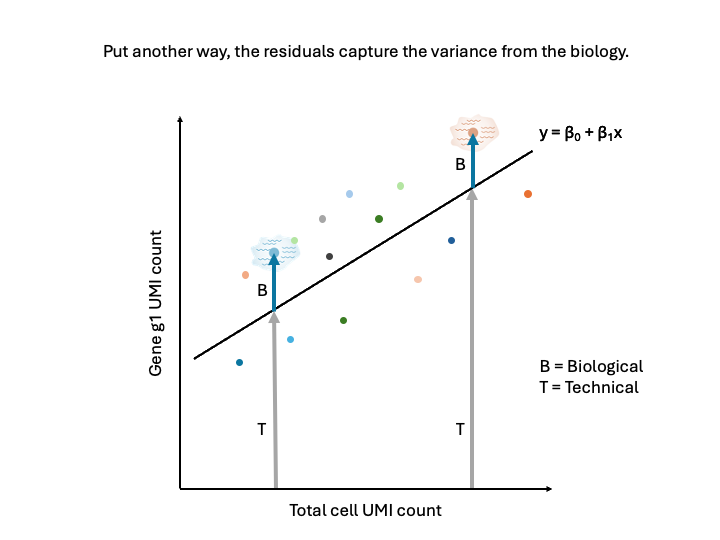
In other words, the residuals represent the biological variance, and the regression removes the technical variance. Note now that the residuals are the about the same for the two cells.
Additional details
The full description and justification of the
SCTransform() function are provided in two excellent
papers:
Hafemeister & Satija, Normalization and variance stabilization of single-cell RNA-seq data using regularized negative binomial regression, 2019, Genome Biology (link)
Choudhary & Satija, Comparison and evaluation of statistical error models for scRNA-seq, 2022, Genome Biology (link)
A benefit of the this framework for normalization is that the model
can include other terms which can account for unwanted technical
variation. One example of this is the percent mitochondrial reads
(percent.mt). The vars.to.regress parameter of
SCTransform() is used for this purpose. See the documentation
for details.
Other normalizations
From the Seurat documentation, the SCTransform()
function “replaces NormalizeData(),
ScaleData(), and FindVariableFeatures()”. This
chain of functions is referred to as the “log-normalization procedure”.
You may see these three commands in other vignettes, and even in other
Seurat vignettes (source).
In the two papers referenced above, the authors show how the
log-normalization procedure does not always fully account for cell
sequencing depth and overdispersion. Therefore, we urge you to use this
alternative pipeline with caution.
Normalization, continued
By now, SCTransform() should have finished running, so
let’s take a look at the result:
# -------------------------------------------------------------------------
# Consider the new SCT layer and examine Seurat Object
Assays(geo_so)
[1] "RNA" "SCT"geo_soAn object of class Seurat
46957 features across 31559 samples within 2 assays
Active assay: SCT (20468 features, 3000 variable features)
3 layers present: counts, data, scale.data
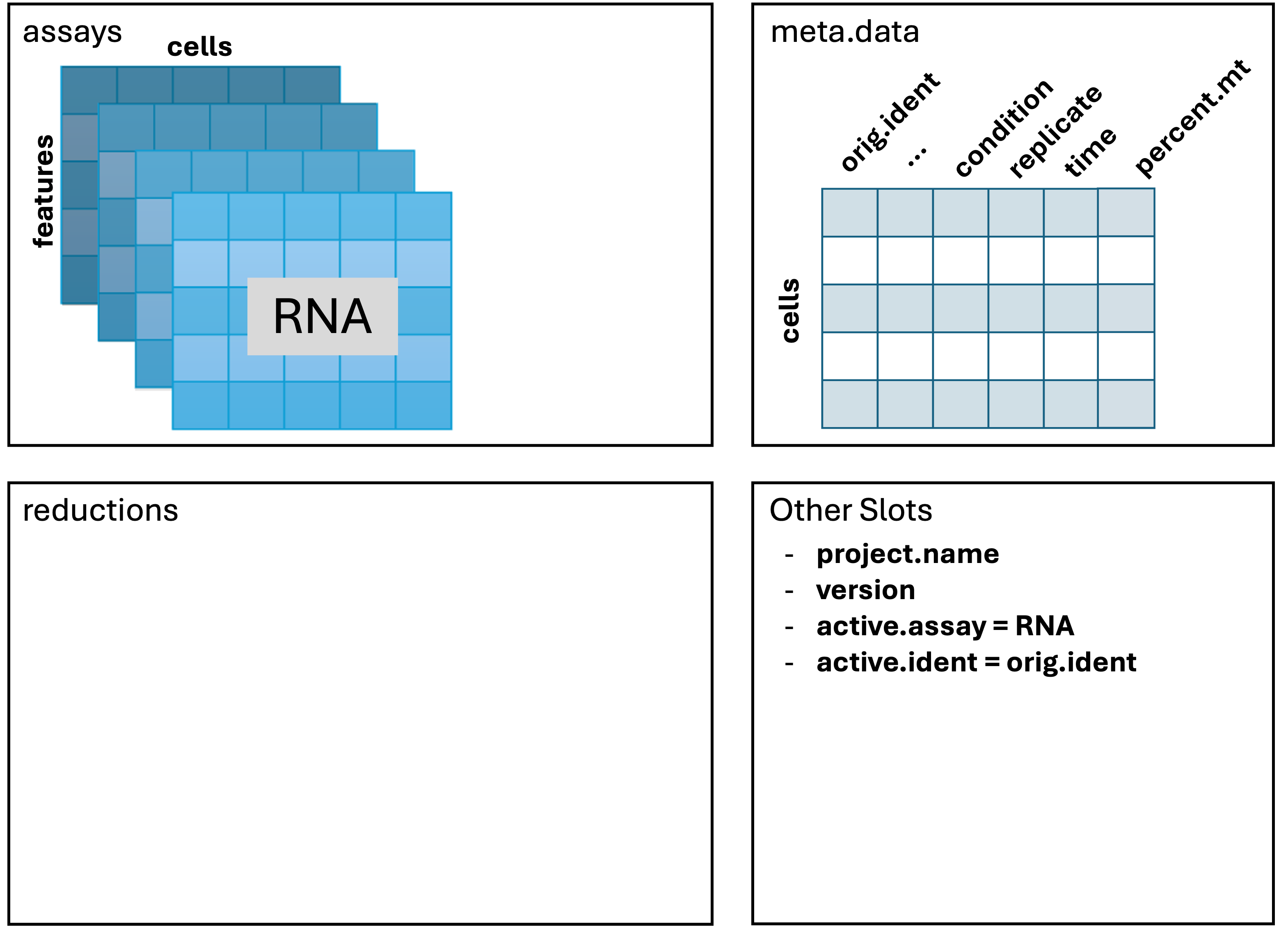
1 other assay present: RNAThe Seurat object now looks like this:
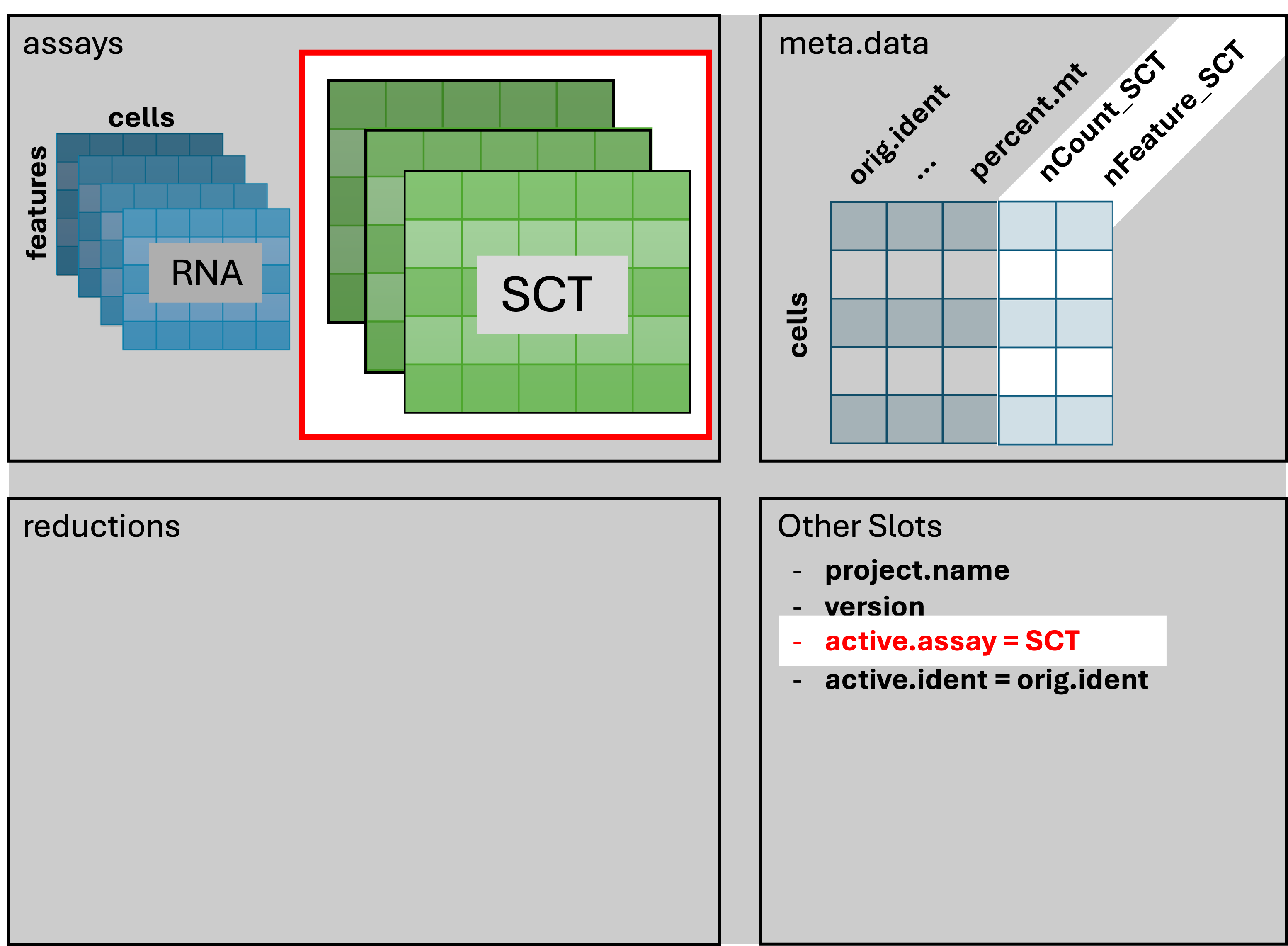
- Note additional columns in
meta.dataand the change of theactive.assayto SCT.
SCT Assay Layers
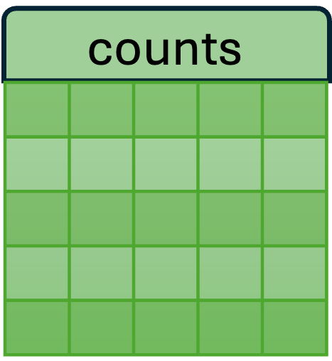
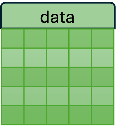
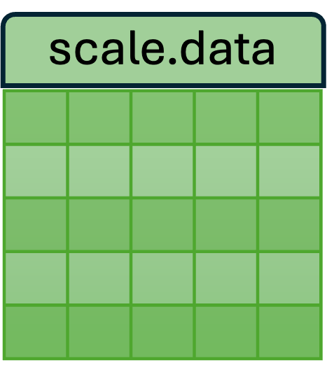
- The new SCT assay has three layers: counts, data, and scale.data.
- Each of these layers is a matrix of cells (columns) x genes (rows) x values.
 |
 |
 |
|---|---|---|
| Used for differential expression analysis (which generally require count data). | Log of counts; used for visualization. | Used by the downstream PCA, UMAP, and clustering analyses. |
How SCTransform builds each layer
To understand how SCTranform derives the new SCT layers,
it helps to consider a single gene (e.g. C1qb) of a single
sample (HODay0replicate1).

A. SCTransform() begins with the observed RNA counts.
This plot shows the cell UMI depth vs the counts for a single gene
(C1qb). Each dot is a cell; the axes are log-log scaled.
B. For each measured gene, SCTransform() fits a model to
the observed RNA counts and determines the median cell depth (the light
blue curve and red vertical line respectively in plot A above). The
fitted model shows that cells with higher depth show higher expression
for this gene; this is likely not biological and instead a
technical effect due to the reaction efficiency of the cell in
protocol.
C. scale.data : Applying the model to the observed counts, the residuals (the difference between the model and observed) are stored in the scale.data matrix. These residuals are scaled so that the expression patterns from low-expressing genes can be compared with patterns from high-expressing genes.
D. counts : Using the scale.data results and the
median cell depth for this gene (highlighted in plot A),
SCTransform() runs the model “in reverse” to create a set
of corrected counts. The corrected counts effectively remve the
cell-specific technical effect.
E. data : The counts matrix is log transformed to become the data matrix. The fitted line (light green) is flat, indicating the cell-specific technical effects have been removed.
Again, the plots above are focused on one gene and one sample (representing a subset of measured cells), so these results would represent the “first part” of a single row of these new SCT matrices. After fitting a model on all genes and all samples we get three full SCT matrices shown above.
Save our progress
Let’s save this normalized form of our Seurat object.
# -------------------------------------------------------------------------
# Save Seurat object
saveRDS(geo_so, file = 'results/rdata/geo_so_sct_normalized.rds')
Once that completes, we’ll power down the session.
Summary
|
|
| The counts in the feature barcode matrix are a blend of technical and biological effects. Technical effects can distort or mask the biological effects of interest, confounding downstream analyses. Seurat can model the technical effects based on overall patterns in expression across all cells. Once these technical effects are minimized, the remaining signal is primarily due to biological variance. |
In this section we have run the SCTransform() function
to account for variation in cell sequencing depth and to stabilize the
variance of the counts.
Next steps: PCA and integration
These materials have been adapted and extended from materials listed above. These are open access materials distributed under the terms of the Creative Commons Attribution license (CC BY 4.0), which permits unrestricted use, distribution, and reproduction in any medium, provided the original author and source are credited.
| Previous lesson | Top of this lesson | Next lesson |
|---|