Differential Expression Analysis
UM Bioinformatics Core Workshop Team
2025-10-16
Workflow Overview
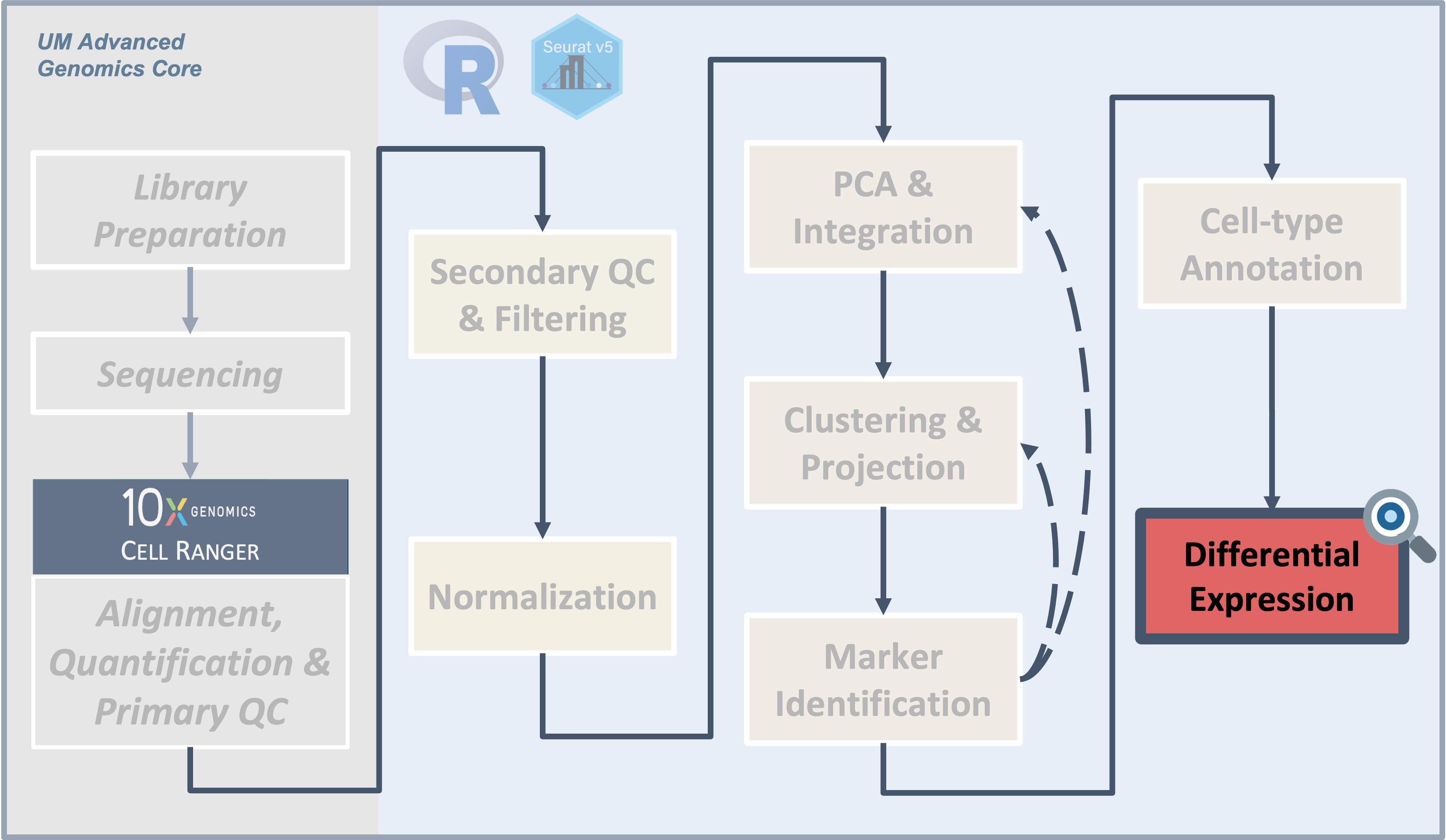
Introduction
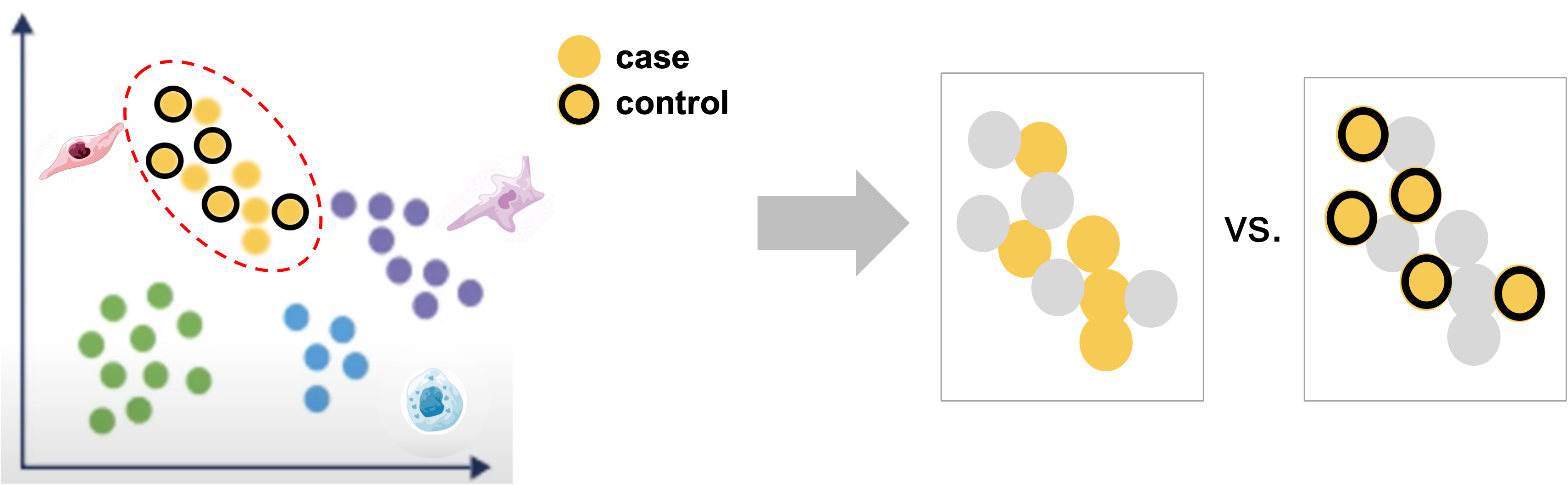
|
| Starting with labeled clustered data, for each labeled cluster, we can compare between case and control within that cluster to identify genes that are impacted by the experimental perturbation(s) for that cell-type or subtype. |
After identifying what cell-types are likely present in our data, we
can finally consider experimental conditions and use differential
expression comparisons to address the biological question at hand for an
experiment.
Objectives
- Run “standard” differential expression comparisons with cells as replicates
- Run “pseudobulk” differential expression comparisons with samples as replicates
We already introduced DE comparisons in the marker identification section of this workshop, but here we will show how to run comparisons between experimental conditions for each annotated cluster.
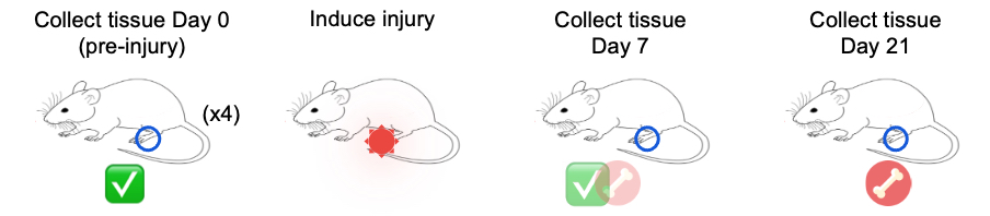
As a reminder, our data includes cells isolated from issue from day 0 (prior to injury) as controls, and days 7 and 21 post-injury as experimental conditions.
Differential Expression
For single-cell data there are generally two types approaches for running differential expression - either a cell-level or sample-level approach.
For cell-level comparisons, simpler statistical methods like a t-test or the Wilcoxon rank-sum test or single-cell specific methods that models cells individually like MAST can be used.
As mentioned earlier, many of the tools developed for bulk RNA-seq have been shown to have good performance for single-cell data, such as EdgeR or DESeq2, particularly when the count data is aggregated into sample-level “pseudobulk” values for each cluster source.
As discussed in the single-cell best practices book there are active benchmarking efforts and threshold considerations for single-cell data.
Standard comparisons
First we’ll run cell-level comparisons for our data for the pericyte
cluster, which seemed to have an interesting pattern between time points
in the UMAP plots, starting with cells from the D21 vs D7 conditions.
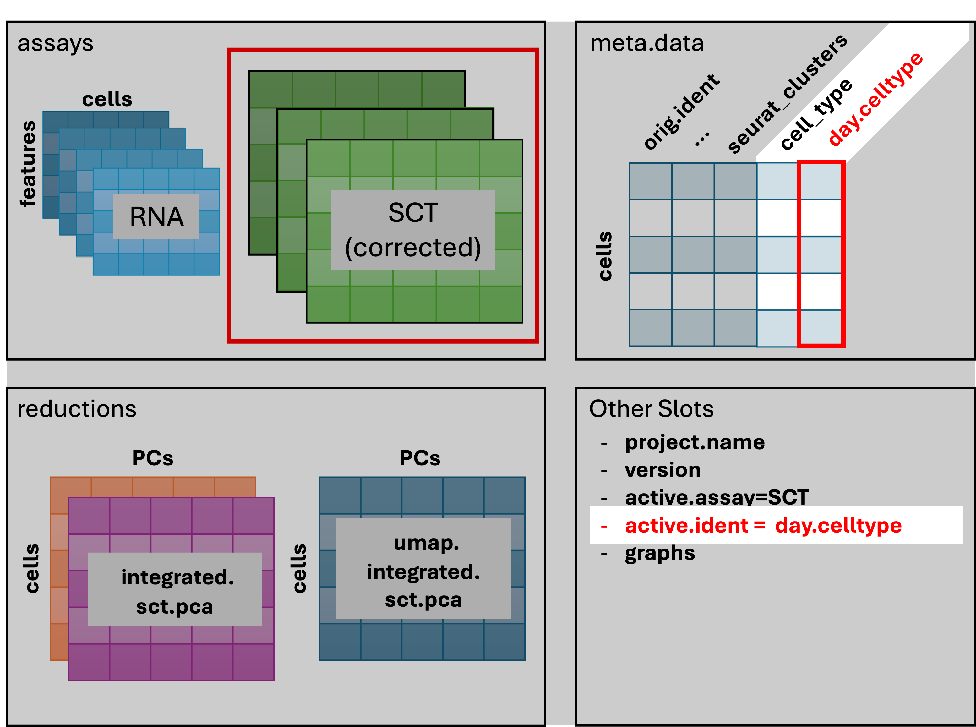
We’ll need to ensure our cells are labeled to reflect both the cluster
and condition identities before running our comparison using
FindMarker() and summarizing the results:
# =========================================================================
# Differential Expression Analysis
# =========================================================================

# Create combined label of day + celltype to use for DE contrasts
geo_so$day.celltype = paste(geo_so$time, geo_so$cell_type, sep = '_')
# check labels
unique(geo_so$day.celltype)
[1] "Day0_Myofibroblast" "Day0_Hematopoietic Stem Cell" "Day0_Dendritic Cell" "Day0_Monocyte" "Day0_B cell"
[6] "Day0_Platelet" "Day0_Smooth muscle cell" "Day0_Stem Cell" "Day0_Pericyte" "Day0_Fibroblast"
[11] "Day0_Unknown" "Day0_T Cell" "Day0_Infl. Macrophage" "Day7_Hematopoietic Stem Cell" "Day7_Dendritic Cell"
[16] "Day7_Monocyte" "Day7_Pericyte" "Day7_Myofibroblast" "Day7_Platelet" "Day7_Infl. Macrophage"
[21] "Day7_Smooth muscle cell" "Day7_Stem Cell" "Day7_Fibroblast" "Day7_B cell" "Day7_T Cell"
[26] "Day7_Unknown" "Day21_Smooth muscle cell" "Day21_Dendritic Cell" "Day21_Monocyte" "Day21_Myofibroblast"
[31] "Day21_Pericyte" "Day21_Hematopoietic Stem Cell" "Day21_Fibroblast" "Day21_Platelet" "Day21_T Cell"
[36] "Day21_Stem Cell" "Day21_Infl. Macrophage" "Day21_Unknown" "Day21_B cell" # Reset cell identities to the combined condition + celltype label
Idents(geo_so) = 'day.celltype'| x |
|---|
| Day0_Myofibroblast |
| Day0_Hematopoietic Stem Cell |
| Day0_Dendritic Cell |
| Day0_Monocyte |
| Day0_B cell |
| Day0_Platelet |
| Day0_Smooth muscle cell |
| Day0_Stem Cell |
| Day0_Pericyte |
| Day0_Fibroblast |
| Day0_Unknown |
| Day0_T Cell |
| Day0_Infl. Macrophage |
| Day7_Hematopoietic Stem Cell |
| Day7_Dendritic Cell |
| Day7_Monocyte |
| Day7_Pericyte |
| Day7_Myofibroblast |
| Day7_Platelet |
| Day7_Infl. Macrophage |
| Day7_Smooth muscle cell |
| Day7_Stem Cell |
| Day7_Fibroblast |
| Day7_B cell |
| Day7_T Cell |
| Day7_Unknown |
| Day21_Smooth muscle cell |
| Day21_Dendritic Cell |
| Day21_Monocyte |
| Day21_Myofibroblast |
| Day21_Pericyte |
| Day21_Hematopoietic Stem Cell |
| Day21_Fibroblast |
| Day21_Platelet |
| Day21_T Cell |
| Day21_Stem Cell |
| Day21_Infl. Macrophage |
| Day21_Unknown |
| Day21_B cell |
# -------------------------------------------------------------------------
# Consider pericyte cluster D21 v D7 & run DE comparison using wilcoxon test
de_cell_pericyte_D21_vs_D7 = FindMarkers(
    object = geo_so,
    slot = 'data', test = 'wilcox',
    ident.1 = 'Day21_Pericyte', ident.2 = 'Day7_Pericyte')

head(de_cell_pericyte_D21_vs_D7)
p_val avg_log2FC pct.1 pct.2 p_val_adj
Fmod 5.928788e-323 2.3143072 0.934 0.518 1.213504e-318
Prelp 1.541258e-301 2.6531170 0.760 0.217 3.154647e-297
Gm10076 1.873982e-301 -1.2351650 0.818 0.964 3.835667e-297
Cilp2 1.170085e-283 5.8112649 0.418 0.014 2.394930e-279
Tpt1 9.251339e-282 0.7933017 0.998 0.981 1.893564e-277
Wfdc1 3.601155e-265 6.2241539 0.372 0.006 7.370845e-261# -------------------------------------------------------------------------
# Add gene symbols names and save
# Add rownames as a column for output
de_cell_pericyte_D21_vs_D7$gene = rownames(de_cell_pericyte_D21_vs_D7)
# save to file
write_csv(de_cell_pericyte_D21_vs_D7,
file = 'results/tables/de_standard_pericyte_D21_vs_D7.csv')
# summarize diffex results
table(de_cell_pericyte_D21_vs_D7$p_val_adj < 0.05 &
abs(de_cell_pericyte_D21_vs_D7$avg_log2FC) > log2(1.5))
FALSE  TRUE
 7800  1913
In the first 3 lines of the above code block we can see the changes to the schematic:
Note - the avg_log2FC threshold of 1.5 we use here are
quite stringent as the default log2FC threshold for the function is
0.25. However the default threshold corresponds to only a 19% difference
in RNA levels, which is quite permissive.
If there is enough time - we can also compare between cells from the D7 and D0 conditions within the pericyte population.
# -------------------------------------------------------------------------
# Compare pericyte cluster D7 v D0
de_cell_pericyte_D7_vs_D0 = FindMarkers(
    object = geo_so,
    slot = 'data', test = 'wilcox',
    ident.1 = 'Day7_Pericyte', ident.2 = 'Day0_Pericyte')

head(de_cell_pericyte_D7_vs_D0)
p_val avg_log2FC pct.1 pct.2 p_val_adj
Chad 6.710617e-304 -10.136834 0.002 0.522 1.373529e-299
Cilp2 1.019148e-282 -7.834071 0.014 0.754 2.085992e-278
Ptx4 1.193446e-261 -7.268218 0.005 0.551 2.442744e-257
Chodl 6.033985e-243 -7.172540 0.006 0.536 1.235036e-238
Myoc 1.921030e-188 -9.424580 0.002 0.348 3.931963e-184
Crispld1 8.254509e-153 -7.185990 0.010 0.449 1.689533e-148# -------------------------------------------------------------------------
# Add rownames for D7 v D0 results
de_cell_pericyte_D7_vs_D0$gene = rownames(de_cell_pericyte_D7_vs_D0)
# save to file
write_csv(de_cell_pericyte_D7_vs_D0,
file = 'results/tables/de_standard_pericyte_D7_vs_D0.csv')
# summarize results
table(de_cell_pericyte_D7_vs_D0$p_val_adj < 0.05 &
abs(de_cell_pericyte_D7_vs_D0$avg_log2FC) > log2(1.5))
FALSE  TRUE
10594  1324
This same approach can be extended to run pairwise comparisons between conditions for each annotated cluster of interest.
Pseudobulk comparisons
With advances in the technology as well as decreased sequencing costs allowing for larger scale single-cell experiments (that include replicates), along with a study by Squair et al (2021) that highlighted the possibility of inflated false discovery rates for the cell-level approaches since cells isolated from the same sample are unlikely to be statistically independent source the use of sample-level or “psuedobulk” can be advantageous.
We’ll run psuedobulk comparisons for our data for the pericyte
cluster, starting with the D21 vs D7 conditions. We’ll need to generate
the aggregated counts first (ensuring that we are grouping cells by
replicate labels), before labeling the cells to reflect the cluster and
condition. Then we will run our comparison using
FindMarker() but specifying DESeq2 as our method before
summarizing the results:
# -------------------------------------------------------------------------
# Create pseudobulk object
pseudo_catch_so =
  AggregateExpression(geo_so,
                      assays = 'RNA',
                      return.seurat = TRUE,
                      group.by = c('cell_type', 'time', 'replicate'))

# Set up labels to use for comparisons & assign as cell identities
pseudo_catch_so$day.celltype = paste(pseudo_catch_so$time, pseudo_catch_so$cell_type, sep = '_')
Idents(pseudo_catch_so) = 'day.celltype'
# -------------------------------------------------------------------------
# Run pseudobulk comparison between Day 21 and Day 0, using DESeq2
de_pseudo_pericyte_D21_vs_D7 = FindMarkers(
object = pseudo_catch_so,
ident.1 = 'Day21_Pericyte', ident.2 = 'Day7_Pericyte',
test.use = 'DESeq2')
# Take a look at the table
head(de_pseudo_pericyte_D21_vs_D7) p_val avg_log2FC pct.1 pct.2 p_val_adj
Cilp2 3.861291e-232 2.906378 1 1 1.022817e-227
Ltbp4 5.631946e-118 1.712277 1 1 1.491846e-113
Cd55 1.853515e-95 1.290895 1 1 4.909776e-91
Prss23 2.598750e-87 1.644203 1 1 6.883828e-83
Nav3 3.019557e-87 -1.594133 1 1 7.998504e-83
Gm42418 7.456053e-82 2.249675 1 1 1.975034e-77# -------------------------------------------------------------------------
# add genes rownames as a column for output
de_pseudo_pericyte_D21_vs_D7$gene = rownames(de_pseudo_pericyte_D21_vs_D7)
# save results
write_csv(de_pseudo_pericyte_D21_vs_D7,
file = 'results/tables/de_pseudo_pericyte_D21_vs_D7.csv')
# review pseudobulk results, using the same thresholds
table(de_pseudo_pericyte_D21_vs_D7$p_val_adj < 0.05 &
abs(de_pseudo_pericyte_D21_vs_D7$avg_log2FC) > log2(1.5))
FALSE  TRUE
23124   483
Since we’re working with pseudobulk data, unlike in the marker identification section, there is no percentage of cells expressing that needs to be represented, so we can summarize our DE results with a volcano plot:
# -------------------------------------------------------------------------
# Make a volcano plot of pseudobulk diffex results
pseudo_pericyte_D21_vs_D7_volcano =
  ggplot(de_pseudo_pericyte_D21_vs_D7, aes(x = avg_log2FC, y = -log10(p_val))) +
  geom_point()

ggsave(filename = 'results/figures/volcano_de_pseudo_pericyte_D21_vs_D0.png',
       plot = pseudo_pericyte_D21_vs_D7_volcano,
       width = 7, height = 7, units = 'in')

pseudo_pericyte_D21_vs_D7_volcano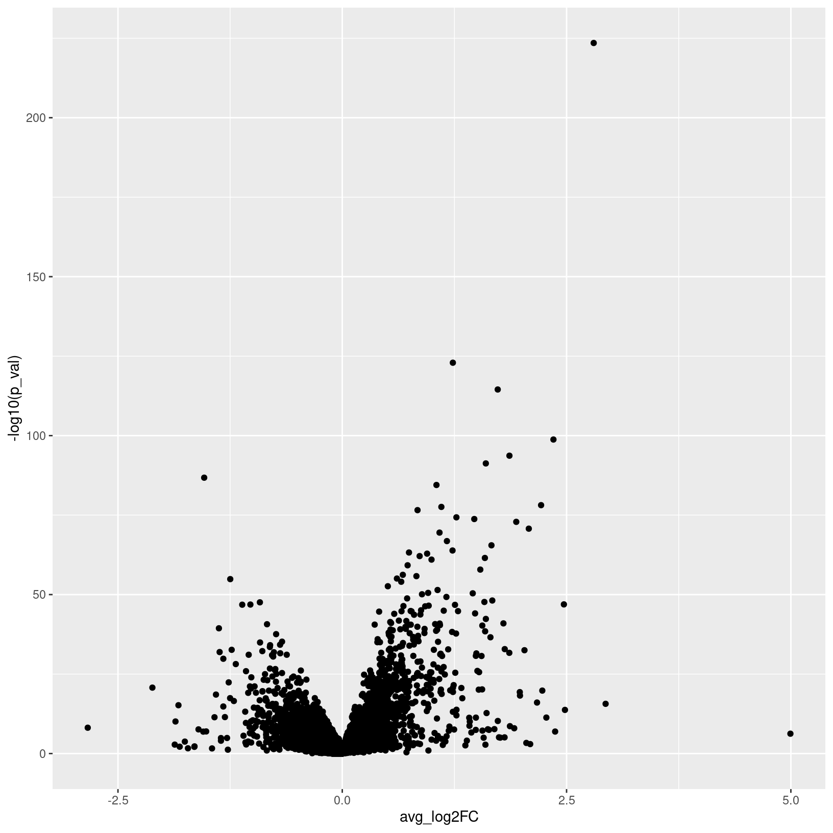
Further examining DE results
We can also overlay the expression of interesting differentially
expressed genes back onto our UMAP plots to highlight the localization
and possible function, again using the FeaturePlot
function.
# -------------------------------------------------------------------------
# UMAP feature plot of Cd55 gene
FeaturePlot(geo_so, features = "Cd55", split.by = "time")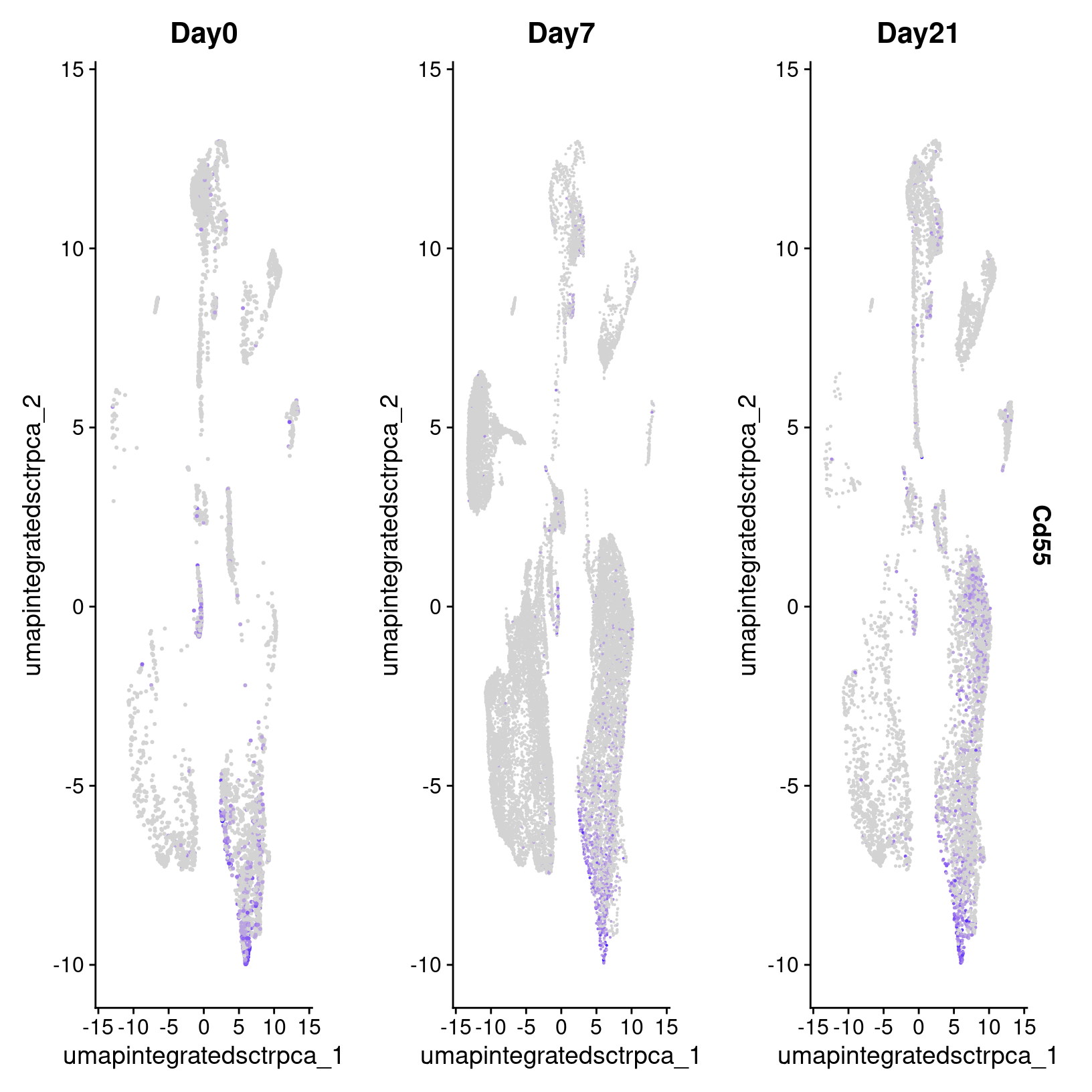 So we found Cd55 based on differential expression comparison in the
Pericyte population between Day 7 and Day 21 but in looking at the
Feature plot of expression, we also see high expression in a subset of
cells on Day 0. This interesting, since according to Shin
et al (2019), CD55 regulates bone mass in mice.
So we found Cd55 based on differential expression comparison in the
Pericyte population between Day 7 and Day 21 but in looking at the
Feature plot of expression, we also see high expression in a subset of
cells on Day 0. This interesting, since according to Shin
et al (2019), CD55 regulates bone mass in mice.
It also looks like there is a high percentage of expression in some of the other precursor populations on the top right of our plots, which is interesting and might suggest an interesting subpopulation that we might try to identify, particularly given the role of this gene and our interest in determining why abberant bone can form after injury.
Next steps
While looking at individual genes can reveal interesting patterns like in the case of Cd55, it’s not a very efficient process. So after running ‘standard’ and/or psuedobulk differential expression comparisons, we can use the same types of tools used downstream of bulk RNA-seq to interpret these results, which we’ll touch on in the next section.
Save our progress
# -------------------------------------------------------------------------
# Discard all ggplot objects currently in environment
# (Ok since we saved the plots as we went along.)
rm(list=names(which(unlist(eapply(.GlobalEnv, is.ggplot)))));
gc()
used (Mb) gc trigger (Mb) max used (Mb)
Ncells 9492623 507.0 17984245 960.5 12351778 659.7
Vcells 348315415 2657.5 795005255 6065.5 792577216 6046.9We’ll save a copy of the final Seurat object to final.
# -------------------------------------------------------------------------
# Save Seurat object
saveRDS(geo_so, file = 'results/rdata/geo_so_sct_integrated_final.rds')
Summary
|
|
| Starting with labeled clustered data, for each labeled cluster, we can compare between case and control within that cluster to identify genes that are impacted by the experimental perturbation(s) for that cell-type or subtype. |
Reviewing these results should allow us to identify genes of interest that are impacted by injury and in the context of the cell-types in which they are differentially expressed, formalize some hypotheses for what cell-types or biological processes might be contributing to aberrant bone formation.
These materials have been adapted and extended from materials listed above. These are open access materials distributed under the terms of the Creative Commons Attribution license (CC BY 4.0), which permits unrestricted use, distribution, and reproduction in any medium, provided the original author and source are credited.
| Previous lesson | Top of this lesson | Analysis Summary |
|---|