Exercises - Intro to Single-Cell Analysis

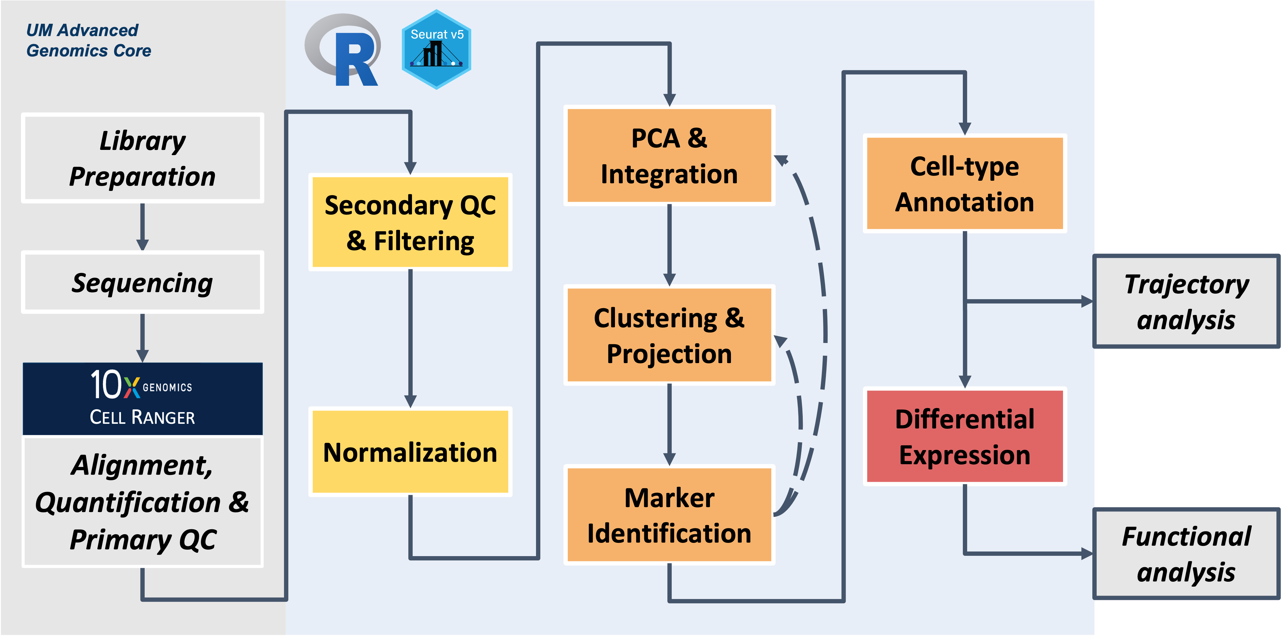
Workflow Overview

Workshop exercises

Build on the content and analysis steps covered in the workshop sessions by working through these independent exercises. Note - if you work on the exercises make sure to restart R session to clear out environment before closing the window (like we have at the end of each session) to avoid lags when logging in the next day

---

Reminder: RStudio, Seurat, and Memory Management

• R and RStudio are designed to grab computer memory (RAM) when necessary and release that memory when it’s no longer needed. R does this with a fancy computer science technique called garbage collection.

• The R garbage collector is very good for small objects and simple analyses, but complex single-cell analysis can overwhelm it. So don’t rely on R/RStudio’s built in garbage collection and session management for single-cell analysis. Instead, do the following:

---

1. Save intermediate versions of the Seurat object as you go along using saveRDS(). This gives you “savepoints” so if you need to backtrack, you don’t have to go back to the beginning.
   
2. Save ggplots into image files as you go along. Periodically clear ggplot objects from the R environment.
   
3. At the end of each day, wherever you are in the analysis, explicitly save the Seurat object and “power down” your session.
   
4. The next day, you can load the Seruat object using readRDS().
   

---

This simple pattern will make your code more reproducible and your RStudio session more reliable.

Day 1

You don’t need to have a fresh environment for these exercises. All variable names will be different from the lessons. Load the libraries (it’s okay if they’re already loaded) and the unfiltered Seurat object with the following code:

# =========================================================================
# Independent Exercise - Day 1 Startup
# =========================================================================

# After restarting our R session, load the required libraries & input data
library(Seurat)
library(BPCells)
library(tidyverse)

# Use provided copy of integrated data
exso = readRDS('./inputs/prepared_data/rdata/geo_so_unfiltered.rds')

# Add percent.mt column to meta.data
exso$percent.mt = PercentageFeatureSet(exso, pattern = '^mt-')

## NOTE - BEFORE STOPPING WORK ON THE EXERCISES REMEMBER TO POWER DOWN AND RESTART R SESSION !!!!

Let’s practice filtering cells based on different criteria than we’re using in the lessons.

Day 1 Exercise 1

Subset exso so that all cells have nFeature_RNA greater than or equal to 1000. How many cells remain?

Hint 1: For a reminder of how to subset a Seurat object, see the “Removing low-quality cells” section of the Secondary QC and Filtering module. Hint 2: For a reminder, of how to count the number cells per sample, see the “Cell counts” section of the Secondary QC and Filtering module.

Day 1 Exercise 2

Subset exso so that all cells have nCount_RNA greater than or equal to 5000. How many cells remain?

Day 1 Exercise 3

Subset exso so that all cells have percent.mt less than 10%. How many cells remain?

Day 1 Exercise 4

Subset exso so that each of the previous three conditions are satisfied. How many cells remain?

Day 1 solutions

Scripts

# =========================================================================
# Independent Exercise - Day 1 Startup
# =========================================================================

# After restarting our R session, load the required libraries & input data
library(Seurat)
library(BPCells)
library(tidyverse)

# Load the unfiltered version and give it a new variable name
exso = readRDS('./inputs/prepared_data/rdata/geo_so_unfiltered.rds')

# Add percent.mt column to meta.data
exso$percent.mt = PercentageFeatureSet(exso, pattern = '^mt-')

## NOTE - BEFORE STOPPING WORK ON THE EXERCISES REMEMBER TO POWER DOWN AND RESTART R SESSION !!!!

# Exercise 1
exso = subset(exso, nFeature_RNA >= 1000)

ex1 = exso@meta.data %>% count(orig.ident, name = 'postfilter_cells')
ex1

# Exercise 2
exso = subset(exso, nCount_RNA >= 1000)

ex2 = exso@meta.data %>% count(orig.ident, name = 'postfilter_cells')
ex2

# Exercise 3
exso = subset(exso, percent.mt < 10)

ex3 = exso@meta.data %>% count(orig.ident, name = 'postfilter_cells')
ex3

# Exercise 4
exso = subset(exso, nFeature_RNA >= 1000 & nCount_RNA >= 1000 & percent.mt < 10)

ex4 = exso@meta.data %>% count(orig.ident, name = 'postfilter_cells')
ex4

Full output

# =========================================================================
# Independent Exercise - Day 1 Startup
# =========================================================================

# After restarting our R session, load the required libraries & input data
library(Seurat)
library(BPCells)
library(tidyverse)

# Load the unfiltered version and give it a new variable name
exso = readRDS('./inputs/prepared_data/rdata/geo_so_unfiltered.rds')

# Add percent.mt column to meta.data
exso$percent.mt = PercentageFeatureSet(exso, pattern = '^mt-')

## NOTE - BEFORE STOPPING WORK ON THE EXERCISES REMEMBER TO POWER DOWN AND RESTART R SESSION !!!!

# Exercise 1
exso = subset(exso, nFeature_RNA >= 1000)

ex1 = exso@meta.data %>% count(orig.ident, name = 'postfilter_cells')
ex1

          orig.ident postfilter_cells
1   HODay0replicate1              937
2   HODay0replicate2              545
3   HODay0replicate3              992
4   HODay0replicate4              833
5  HODay21replicate1             1854
6  HODay21replicate2             1094
7  HODay21replicate3             1093
8  HODay21replicate4             2288
9   HODay7replicate1             3756
10  HODay7replicate2             4212
11  HODay7replicate3             4207
12  HODay7replicate4             3445

# Exercise 2
exso = subset(exso, nCount_RNA >= 1000)

ex2 = exso@meta.data %>% count(orig.ident, name = 'postfilter_cells')
ex2

          orig.ident postfilter_cells
1   HODay0replicate1              937
2   HODay0replicate2              545
3   HODay0replicate3              992
4   HODay0replicate4              833
5  HODay21replicate1             1854
6  HODay21replicate2             1094
7  HODay21replicate3             1093
8  HODay21replicate4             2288
9   HODay7replicate1             3756
10  HODay7replicate2             4212
11  HODay7replicate3             4207
12  HODay7replicate4             3445

# Exercise 3
exso = subset(exso, percent.mt < 10)

ex3 = exso@meta.data %>% count(orig.ident, name = 'postfilter_cells')
ex3

          orig.ident postfilter_cells
1   HODay0replicate1              886
2   HODay0replicate2              535
3   HODay0replicate3              976
4   HODay0replicate4              821
5  HODay21replicate1             1793
6  HODay21replicate2             1059
7  HODay21replicate3             1052
8  HODay21replicate4             2179
9   HODay7replicate1             3574
10  HODay7replicate2             4057
11  HODay7replicate3             4069
12  HODay7replicate4             3299

# Exercise 4
exso = subset(exso, nFeature_RNA >= 1000 & nCount_RNA >= 1000 & percent.mt < 10)

ex4 = exso@meta.data %>% count(orig.ident, name = 'postfilter_cells')
ex4

          orig.ident postfilter_cells
1   HODay0replicate1              886
2   HODay0replicate2              535
3   HODay0replicate3              976
4   HODay0replicate4              821
5  HODay21replicate1             1793
6  HODay21replicate2             1059
7  HODay21replicate3             1052
8  HODay21replicate4             2179
9   HODay7replicate1             3574
10  HODay7replicate2             4057
11  HODay7replicate3             4069
12  HODay7replicate4             3299

---

Day 2

Since we are working with larger object sizes, it’s best to start with a fresh session. All variable names will be different from the lessons. Load the libraries (it’s okay if they’re already loaded) and the integrated Seurat object with the following code:

# =========================================================================
# Independent Exercise - Day 2 Startup
# =========================================================================

# After restarting our R session, load the required libraries & input data
library(Seurat)
library(BPCells)
library(tidyverse)

# Use provided copy of integrated data
exso2 = readRDS('inputs/prepared_data/rdata/geo_so_sct_integrated.rds')
exso2 # check that object loaded

## NOTE - BEFORE STOPPING WORK ON THE EXERCISES REMEMBER TO POWER DOWN AND RESTART R SESSION !!!!

Day 2 Exercise 1 - Clustering with reduced number of PCs

Test how the clustering results would change if you used fewer or more PCs when clustering these data.

# -------------------------------------------------------------------------
# Testing fewer PCs for clustering 

# look at elbow plot to check PCs and consider alternatives to the number selected for main materials
ElbowPlot(exso2, ndims = 50, reduction = 'unintegrated.sct.pca')

# select alternative value to try (choose a number <10 or >10 PCs)
pcs = # Your value here #

# generate nearest neighbor (graph), using selected number of PCs
exso2 = FindNeighbors(exso2, dims = 1:pcs, reduction = 'integrated.sct.rpca')

After generating clustering, set resolution parameter - remember this only impacts the how the boundaries of the neighbors are drawn, not the underlying NN graph/structure.

# -------------------------------------------------------------------------
# Testing resolution options to see impact

# start with one resolution
res = # Your value here #

# generate clusters, using `pcs` and `res` to make a custom cluster name that will be added to the metadata
exso2 = FindClusters(exso2, resolution = res, 
                     cluster.name = paste0('int.sct.rpca.clusters', res))

# look at meta.data to see cluster labels
head(exso2@meta.data)

# run UMAP reduction to prepare for plotting
exso2 = RunUMAP(exso2, dims = 1:pcs, 
                  reduction = 'integrated.sct.rpca', 
                  reduction.name = paste0('umap.integrated.sct.rpca_alt', res))

# check object to see if named reduction was added
exso2

Challenge 1: How could we generate clusters for multiple alternative resolutions (e.g. 0.4, 0.8, & 1.0)? Hint - for loops can be useful for iteration in many programming languages, including R.

Day 2 Exercise 2 - Plotting alternative clustering results

After generating our clustering results it’s time to visualize them - create a UMAP plot, ensuring that you generate a UMAP reduction for the appropriate reduction

Hint 1 - Remember the previous code chunk used paste0('umap.integrated.sct.rpca_alt', res)) for the cluster name parameter.

Hint 2 - For a reminder of how to generate a UMAP plot, look at the Visualizing and evaluating clustering from the Clustering and Projection module.

Challenge 2: Create UMAP plots for the alternative resolutions (e.g. 0.4, 0.8, & 1.0) generated in the previous challenge.

Check-in Questions - UMAP for alternative PCs

How does the UMAP plot look when fewer or more PCs are used? Do you notice any relationship between the PC parameter and resolution parameter?

Clean up session

Before closing out the window, make sure to clear environment and restart R session to manage the memory usage

## ----------------------------------------------------------
## Clean up session, including any plot objects
rm(list=names(which(unlist(eapply(.GlobalEnv, is.ggplot)))));
gc()

## Save copy of Seurat object in current state to file
saveRDS(exso2, file = paste0('results/rdata/geo_so_sct_integrated_exercise.rds'))
rm(exso2)
gc()

Day 2 solutions

Scripts

# =========================================================================
# Independent Exercise - Day 2 Startup
# =========================================================================

# After restarting our R session, load the required libraries & input data
library(Seurat)
library(BPCells)
library(tidyverse)

# Use provided copy of integrated data
exso2 = readRDS('inputs/prepared_data/rdata/geo_so_sct_integrated.rds')
exso2 # check that object loaded


### Day 2 Exercise 1 - Clustering with reduced number of PCs
# -------------------------------------------------------------------------
# Testing fewer PCs for clustering 

# look at elbow plot to check PCs and consider alternatives to the number selected for main materials
ElbowPlot(exso2, ndims = 50, reduction = 'unintegrated.sct.pca')

# select alternative value to try (can choose a number <10 or >10 PCs)
pcs = 6

# generate nearest neighbor (graph), using selected number of PCs
exso2 = FindNeighbors(exso2, dims = 1:pcs, reduction = 'integrated.sct.rpca')

# -------------------------------------------------------------------------
# start with one resolution
res = 0.2

# generate clusters, using `pcs` and `res` to make a custom cluster name that will be added to the metadata
exso2 = FindClusters(exso2, resolution = res, 
                     cluster.name = paste0('int.sct.rpca.clusters', res))

# look at meta.data to see cluster labels
head(exso2@meta.data)

# run UMAP reduction to prepare for plotting
exso2 = RunUMAP(exso2, dims = 1:pcs, 
                reduction = 'integrated.sct.rpca', 
                reduction.name = paste0('umap.integrated.sct.rpca_alt', res))

# check object to see if named reduction was added
exso2


## Challenge 1 - solution option
# -------------------------------------------------------------------------
# use for loop to generate clustering with alternative resolutions
for(i in c(0.4, 0.8, 1.0)){
  exso2 = FindClusters(exso2, resolution = i, 
                       cluster.name = paste0('int.sct.rpca.clusters', i))
  
  # look at meta.data to see cluster labels
  head(exso2@meta.data)
  
  # run UMAP reduction to prepare for plotting
  exso2 = RunUMAP(exso2, dims = 1:pcs, 
                  reduction = 'integrated.sct.rpca', 
                  reduction.name = paste0('umap.integrated.sct.rpca_alt', i))
  
  # check object to see if multiple cluster resolutions are added
  head(exso2@meta.data)
}



### Day 2 Exercise 2 - Plotting alternative clustering results
# -------------------------------------------------------------------------
# plot clustering results
post_integration_umap_clusters_testing = 
  DimPlot(exso2, group.by = paste0('int.sct.rpca.clusters', res), label = TRUE, 
          reduction = paste0('umap.integrated.sct.rpca_alt', res)) + NoLegend()
post_integration_umap_clusters_testing # look at plot

# output to file, including the number of PCs and resolution used to generate results
ggsave(filename = paste0('results/figures/umap_int_sct_clusters_exercise_', 
                         pcs,'PC.',res,'res','.png'),
       plot = post_integration_umap_clusters_testing, 
       width = 8, height = 6, units = 'in')


## Challenge 2 - solution option
# -------------------------------------------------------------------------
# use for loop to visualize clustering across tested resolutions
post_integration_umap_plots <- c()
for(i in c(0.4, 0.8, 1.0)){
  res_type = paste0("res_", i)
  post_integration_umap_plots[[res_type]] = 
    DimPlot(exso2, group.by = paste0('int.sct.rpca.clusters', i), label = TRUE, 
            reduction = paste0('umap.integrated.sct.rpca_alt', i)) + NoLegend()
}

# look at plots for each resolution stored in list
post_integration_umap_plots
# remove plot list to clean up session 
rm(post_integration_umap_plots)


## ----------------------------------------------------------
## Clean up session, including any plot objects
rm(list=names(which(unlist(eapply(.GlobalEnv, is.ggplot)))));
gc()

## Save copy of Seurat object in current state to file
saveRDS(exso2, file = paste0('results/rdata/geo_so_sct_clustered_exercise.rds'))
rm(exso2)
gc()

Full output

# =========================================================================
# Independent Exercise - Day 2 Startup
# =========================================================================

# After restarting our R session, load the required libraries & input data
library(Seurat)
library(BPCells)
library(tidyverse)

# Use provided copy of integrated data
exso2 = readRDS('inputs/prepared_data/rdata/geo_so_sct_integrated.rds')
exso2 # check that object loaded

An object of class Seurat 
46957 features across 31559 samples within 2 assays 
Active assay: SCT (20468 features, 3000 variable features)
 3 layers present: counts, data, scale.data
 1 other assay present: RNA
 2 dimensional reductions calculated: unintegrated.sct.pca, integrated.sct.rpca

### Day 2 Exercise 1 - Clustering with reduced number of PCs
# -------------------------------------------------------------------------
# Testing fewer PCs for clustering 

# look at elbow plot to check PCs and consider alternatives to the number selected for main materials
ElbowPlot(exso2, ndims = 50, reduction = 'unintegrated.sct.pca')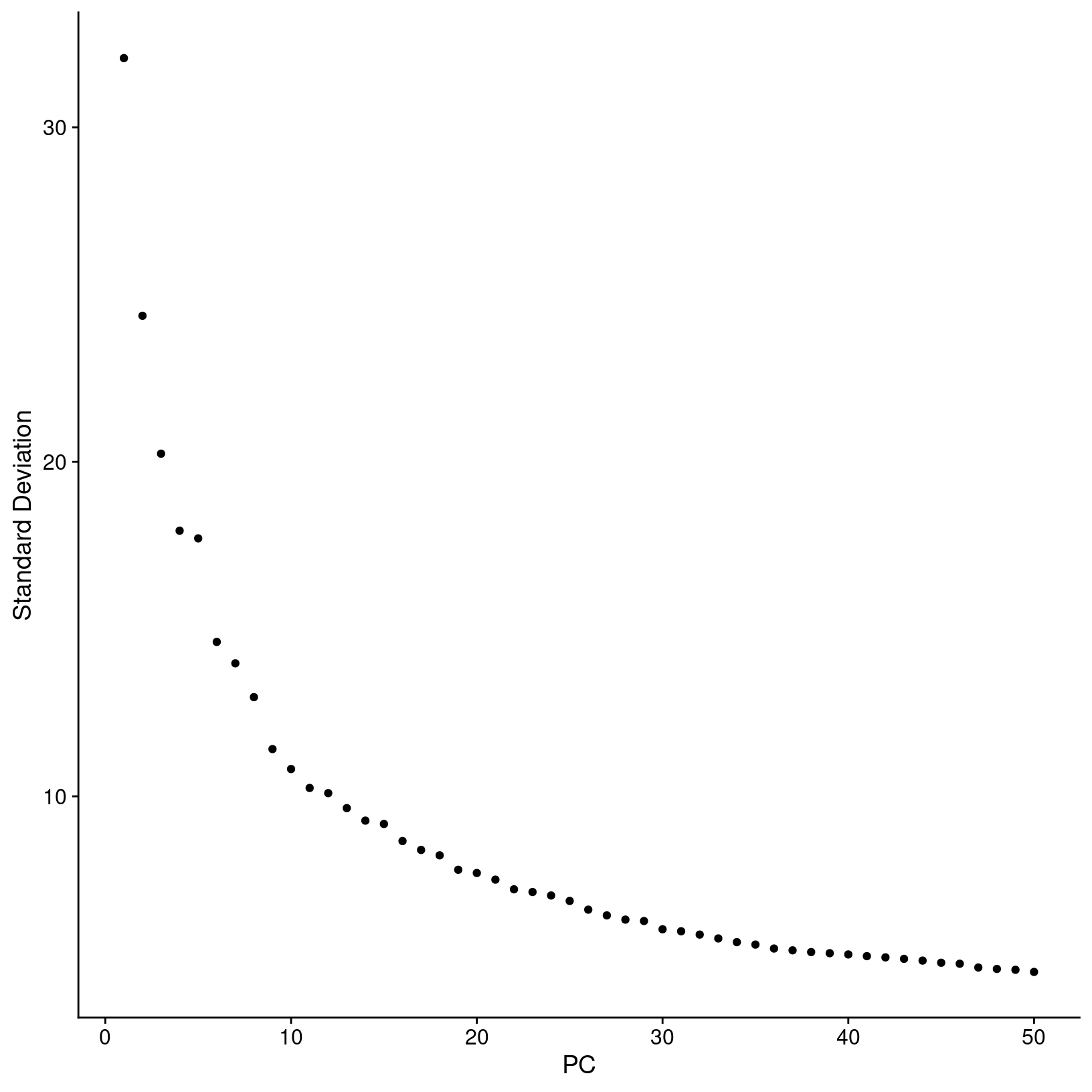

# select alternative value to try (can choose a number <10 or >10 PCs)
pcs = 6

# generate nearest neighbor (graph), using selected number of PCs
exso2 = FindNeighbors(exso2, dims = 1:pcs, reduction = 'integrated.sct.rpca')

Computing nearest neighbor graph

Computing SNN

# -------------------------------------------------------------------------
# start with one resolution
res = 0.2

# generate clusters, using `pcs` and `res` to make a custom cluster name that will be added to the metadata
exso2 = FindClusters(exso2, resolution = res, 
                     cluster.name = paste0('int.sct.rpca.clusters', res))

Modularity Optimizer version 1.3.0 by Ludo Waltman and Nees Jan van Eck

Number of nodes: 31559
Number of edges: 950342

Running Louvain algorithm...
Maximum modularity in 10 random starts: 0.9612
Number of communities: 12
Elapsed time: 3 seconds

# look at meta.data to see cluster labels
head(exso2@meta.data)

                                          orig.ident nCount_RNA nFeature_RNA condition time  replicate percent.mt nCount_SCT nFeature_SCT int.sct.rpca.clusters0.2 seurat_clusters
HODay0replicate1_AAACCTGAGAGAACAG-1 HODay0replicate1      10234         3226        HO Day0 replicate1   1.240962       6062         2867                        0               0
HODay0replicate1_AAACCTGGTCATGCAT-1 HODay0replicate1       3158         1499        HO Day0 replicate1   7.536415       4607         1509                        0               0
HODay0replicate1_AAACCTGTCAGAGCTT-1 HODay0replicate1      13464         4102        HO Day0 replicate1   3.112002       5314         2370                        0               0
HODay0replicate1_AAACGGGAGAGACTTA-1 HODay0replicate1        577          346        HO Day0 replicate1   1.559792       3877         1031                        7               7
HODay0replicate1_AAACGGGAGGCCCGTT-1 HODay0replicate1       1189          629        HO Day0 replicate1   3.700589       4166          915                        0               0
HODay0replicate1_AAACGGGCAACTGGCC-1 HODay0replicate1       7726         2602        HO Day0 replicate1   2.938131       5865         2588                        0               0

# run UMAP reduction to prepare for plotting
exso2 = RunUMAP(exso2, dims = 1:pcs, 
                reduction = 'integrated.sct.rpca', 
                reduction.name = paste0('umap.integrated.sct.rpca_alt', res))

Warning: The default method for RunUMAP has changed from calling Python UMAP via reticulate to the R-native UWOT using the cosine metric
To use Python UMAP via reticulate, set umap.method to 'umap-learn' and metric to 'correlation'
This message will be shown once per session

21:30:02 UMAP embedding parameters a = 0.9922 b = 1.112

21:30:02 Read 31559 rows and found 6 numeric columns

21:30:02 Using Annoy for neighbor search, n_neighbors = 30

21:30:02 Building Annoy index with metric = cosine, n_trees = 50

0%   10   20   30   40   50   60   70   80   90   100%

[----|----|----|----|----|----|----|----|----|----|

**************************************************|
21:30:06 Writing NN index file to temp file /tmp/Rtmp0Y5yMq/file124dae097d3
21:30:06 Searching Annoy index using 1 thread, search_k = 3000
21:30:19 Annoy recall = 100%
21:30:20 Commencing smooth kNN distance calibration using 1 thread with target n_neighbors = 30
21:30:22 Initializing from normalized Laplacian + noise (using RSpectra)
21:30:25 Commencing optimization for 200 epochs, with 1214176 positive edges
21:30:25 Using rng type: pcg
21:30:38 Optimization finished

# check object to see if named reduction was added
exso2

An object of class Seurat 
46957 features across 31559 samples within 2 assays 
Active assay: SCT (20468 features, 3000 variable features)
 3 layers present: counts, data, scale.data
 1 other assay present: RNA
 3 dimensional reductions calculated: unintegrated.sct.pca, integrated.sct.rpca, umap.integrated.sct.rpca_alt0.2

## Challenge 1 - solution option
# -------------------------------------------------------------------------
# use for loop to generate clustering with alternative resolutions
for(i in c(0.4, 0.8, 1.0)){
  exso2 = FindClusters(exso2, resolution = i, 
                       cluster.name = paste0('int.sct.rpca.clusters', i))
  
  # look at meta.data to see cluster labels
  head(exso2@meta.data)
  
  # run UMAP reduction to prepare for plotting
  exso2 = RunUMAP(exso2, dims = 1:pcs, 
                  reduction = 'integrated.sct.rpca', 
                  reduction.name = paste0('umap.integrated.sct.rpca_alt', i))
  
  # check object to see if multiple cluster resolutions are added
  head(exso2@meta.data)
}

Modularity Optimizer version 1.3.0 by Ludo Waltman and Nees Jan van Eck

Number of nodes: 31559
Number of edges: 950342

Running Louvain algorithm...
Maximum modularity in 10 random starts: 0.9428
Number of communities: 20
Elapsed time: 3 seconds

21:30:42 UMAP embedding parameters a = 0.9922 b = 1.112
21:30:42 Read 31559 rows and found 6 numeric columns
21:30:42 Using Annoy for neighbor search, n_neighbors = 30
21:30:42 Building Annoy index with metric = cosine, n_trees = 50
0%   10   20   30   40   50   60   70   80   90   100%
[----|----|----|----|----|----|----|----|----|----|
**************************************************|
21:30:46 Writing NN index file to temp file /tmp/Rtmp0Y5yMq/file124da1abc6065
21:30:46 Searching Annoy index using 1 thread, search_k = 3000
21:30:59 Annoy recall = 100%
21:31:00 Commencing smooth kNN distance calibration using 1 thread with target n_neighbors = 30
21:31:02 Initializing from normalized Laplacian + noise (using RSpectra)
21:31:05 Commencing optimization for 200 epochs, with 1214176 positive edges
21:31:05 Using rng type: pcg
21:31:18 Optimization finished

Modularity Optimizer version 1.3.0 by Ludo Waltman and Nees Jan van Eck

Number of nodes: 31559
Number of edges: 950342

Running Louvain algorithm...
Maximum modularity in 10 random starts: 0.9216
Number of communities: 28
Elapsed time: 3 seconds

21:31:22 UMAP embedding parameters a = 0.9922 b = 1.112
21:31:22 Read 31559 rows and found 6 numeric columns
21:31:22 Using Annoy for neighbor search, n_neighbors = 30
21:31:22 Building Annoy index with metric = cosine, n_trees = 50
0%   10   20   30   40   50   60   70   80   90   100%
[----|----|----|----|----|----|----|----|----|----|
**************************************************|
21:31:26 Writing NN index file to temp file /tmp/Rtmp0Y5yMq/file124da9655b50
21:31:26 Searching Annoy index using 1 thread, search_k = 3000
21:31:39 Annoy recall = 100%
21:31:39 Commencing smooth kNN distance calibration using 1 thread with target n_neighbors = 30
21:31:41 Initializing from normalized Laplacian + noise (using RSpectra)
21:31:44 Commencing optimization for 200 epochs, with 1214176 positive edges
21:31:44 Using rng type: pcg
21:31:58 Optimization finished

Modularity Optimizer version 1.3.0 by Ludo Waltman and Nees Jan van Eck

Number of nodes: 31559
Number of edges: 950342

Running Louvain algorithm...
Maximum modularity in 10 random starts: 0.9136
Number of communities: 30
Elapsed time: 3 seconds

21:32:02 UMAP embedding parameters a = 0.9922 b = 1.112
21:32:02 Read 31559 rows and found 6 numeric columns
21:32:02 Using Annoy for neighbor search, n_neighbors = 30
21:32:02 Building Annoy index with metric = cosine, n_trees = 50
0%   10   20   30   40   50   60   70   80   90   100%
[----|----|----|----|----|----|----|----|----|----|
**************************************************|
21:32:06 Writing NN index file to temp file /tmp/Rtmp0Y5yMq/file124da3bc483b2
21:32:06 Searching Annoy index using 1 thread, search_k = 3000
21:32:19 Annoy recall = 100%
21:32:19 Commencing smooth kNN distance calibration using 1 thread with target n_neighbors = 30
21:32:21 Initializing from normalized Laplacian + noise (using RSpectra)
21:32:24 Commencing optimization for 200 epochs, with 1214176 positive edges
21:32:24 Using rng type: pcg
21:32:37 Optimization finished

### Day 2 Exercise 2 - Plotting alternative clustering results
# -------------------------------------------------------------------------
# plot clustering results
post_integration_umap_clusters_testing = 
  DimPlot(exso2, group.by = paste0('int.sct.rpca.clusters', res), label = TRUE, 
          reduction = paste0('umap.integrated.sct.rpca_alt', res)) + NoLegend()
post_integration_umap_clusters_testing # look at plot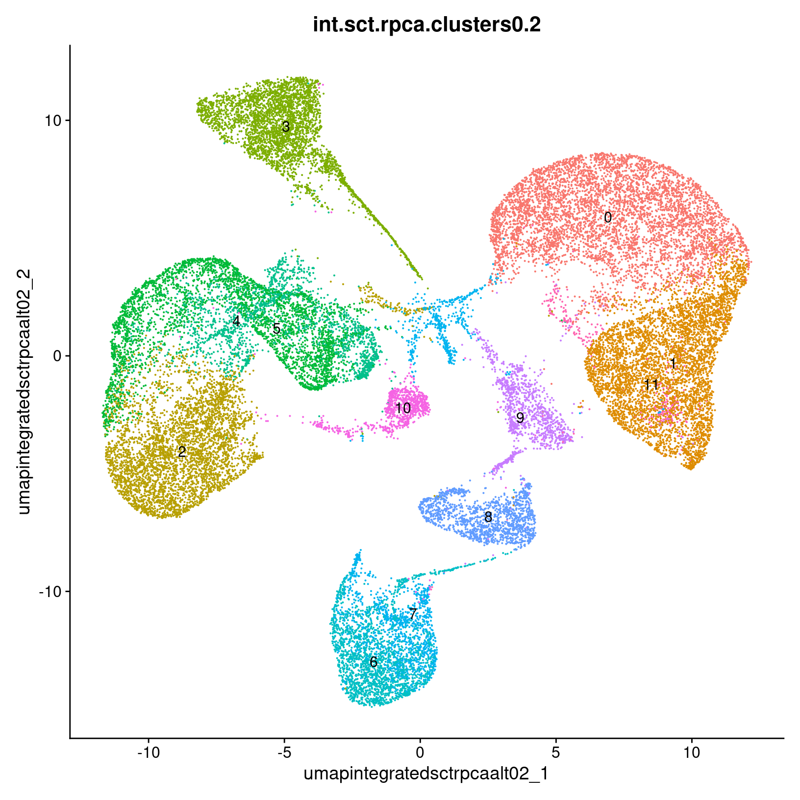

# output to file, including the number of PCs and resolution used to generate results
ggsave(filename = paste0('results/figures/umap_int_sct_clusters_exercise_', 
                         pcs,'PC.',res,'res','.png'),
       plot = post_integration_umap_clusters_testing, 
       width = 8, height = 6, units = 'in')


## Challenge 2 - solution option
# -------------------------------------------------------------------------
# use for loop to visualize clustering across tested resolutions
post_integration_umap_plots <- c()
for(i in c(0.4, 0.8, 1.0)){
  res_type = paste0("res_", i)
  post_integration_umap_plots[[res_type]] = 
    DimPlot(exso2, group.by = paste0('int.sct.rpca.clusters', i), label = TRUE, 
            reduction = paste0('umap.integrated.sct.rpca_alt', i)) + NoLegend()
}

# look at plots for each resolution stored in list
post_integration_umap_plots

$res_0.4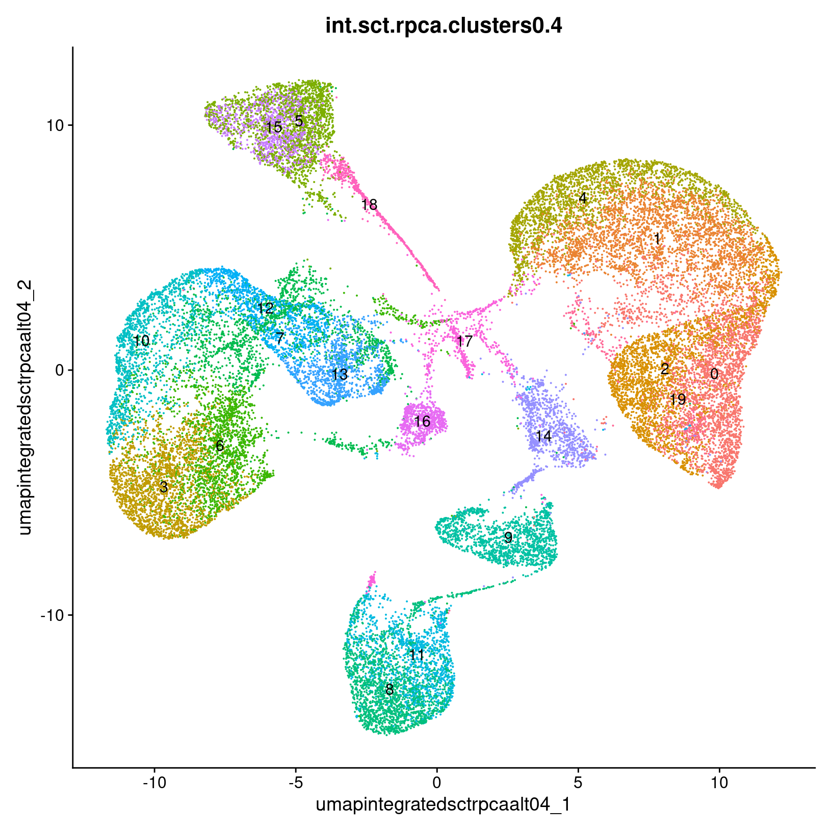

$res_0.8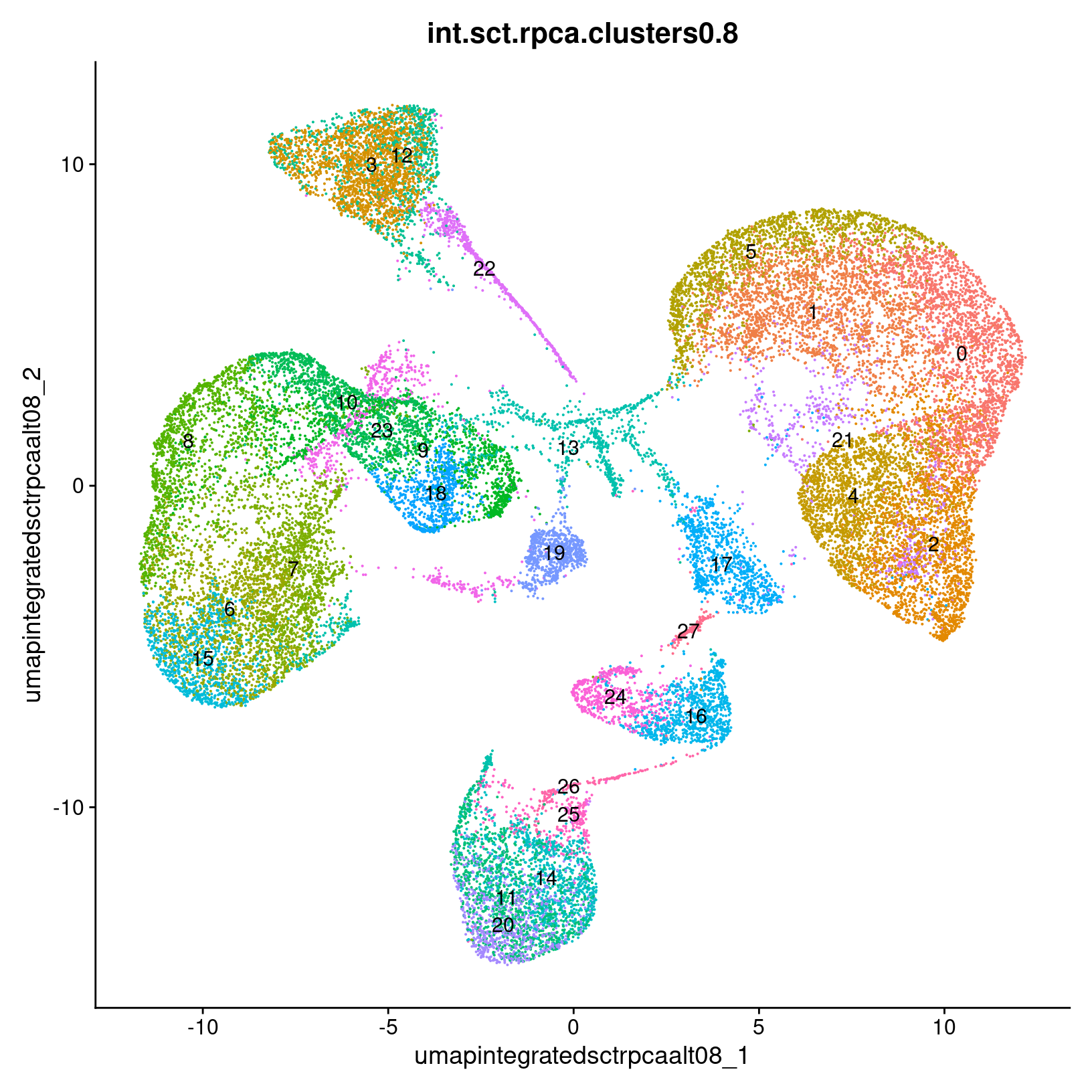

$res_1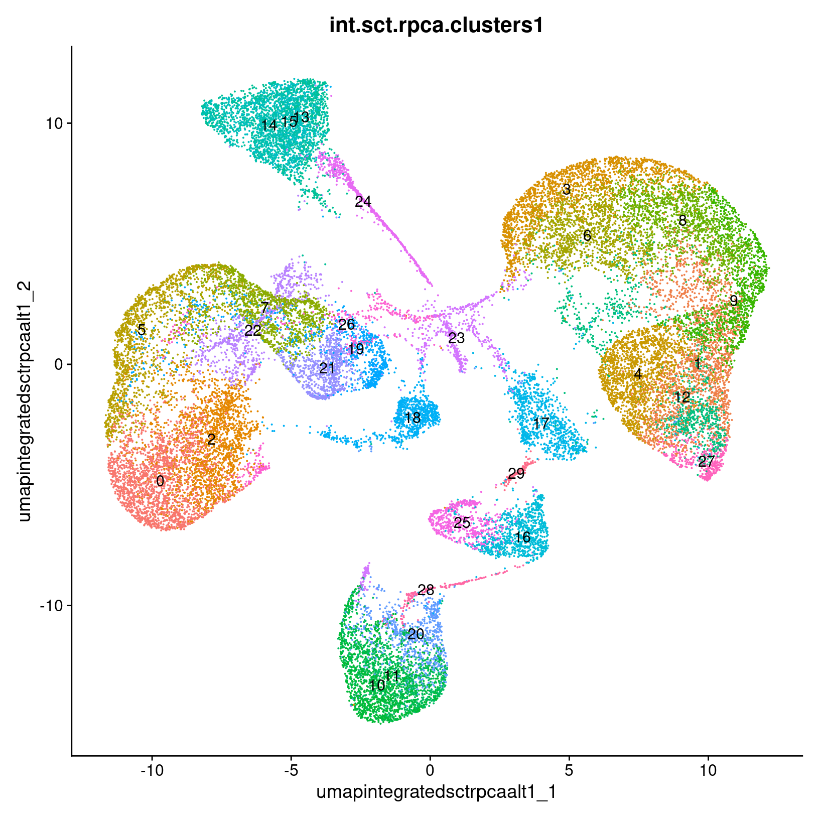

# remove plot list to clean up session 
rm(post_integration_umap_plots)


## ----------------------------------------------------------
## Clean up session, including any plot objects
rm(list=names(which(unlist(eapply(.GlobalEnv, is.ggplot)))));
gc()

            used   (Mb) gc trigger   (Mb)   max used    (Mb)
Ncells   6967048  372.1   10752860  574.3   10752860   574.3
Vcells 384220421 2931.4 1067030484 8140.8 1333787743 10176.0

## Save copy of Seurat object in current state to file
saveRDS(exso2, file = paste0('results/rdata/geo_so_sct_clustered_exercise.rds'))
rm(exso2)
gc()

            used   (Mb) gc trigger   (Mb)   max used    (Mb)
Ncells   6967076  372.1   10752860  574.3   10752860   574.3
Vcells 384236240 2931.5 1067030484 8140.8 1333787743 10176.0

---

Day 3

Since we are working with larger object sizes, it’s best to start with a fresh session. All variable names will be different from the lessons. Load the libraries (it’s okay if they’re already loaded) and a Seurat object with alternative clustering using the following code:

# =========================================================================
# Independent Exercise - Day 3 Startup
# =========================================================================

# After restarting our R session, load the required libraries
library(Seurat)
library(BPCells)
library(tidyverse)
library(scCATCH)

# Load in seurat object with alternative clustering results from yesterday's exercises
exso3 = readRDS('results/rdata/geo_so_sct_integrated_exercise.rds')
exso3 # check that object loaded

## NOTE - BEFORE STOPPING WORK ON THE EXERCISES REMEMBER TO POWER DOWN AND RESTART R SESSION !!!!

Before testing what marker genes and cell-type predictions are generated for an alternative clustering, start by ensuring the Seurat object is set up and has an expected identity set.

## ----------------------------------------------------------
# Check what identities are set
Idents(exso3) %>% head()

pcs = ## use same values as yesterday
res = ## use same values as yesterday

## Set identities to clustering for selected resolution
exso3 = SetIdent(exso3, value = paste0('int.sct.rpca.clusters', res))
Idents(exso3) %>% head()

Day 3 Exercise 1 - examine marker genes for alternative clusters

Using the approach from the marker identification module, run PrepSCTFindMarkers and generate markers for the alternative clustering results. Bonus to generate a table of the top 5 markers and outputing that to file.

Check-in Question - clustering impact on marker genes After you generate markers for the “fewer” pcs option, how do the results differ from the markers found for pcs=10 in the workshop session? What do you think would happen if you tried this with the “more” results?

Day 3 Exercise 2 - Generate predictions for alternative clustering

Using scCATCH like we did for our annotation process, generate predictions for the alternative clustering results.

Day 3 Exercise 3 - Add predictions to Seurat object

Skipping the refinement step, add the cell-type predictions to the Seurat object using the numeric labels as a key, similarly to the our annotation step.

Day 3 Exercise 4 - Plot UMAP with new cluster labels

Using a similar approach used to visualize the annotations in the workshop, generate a UMAP plot

Hint - use the same reduction name as yesterday’s exercise and make sure the group_by parameter matches the column name added to the metadata that stores the predicted cell-types.

Check-in Question

How did the number of pcs and/or resolution change the predictions? Do you think the predictions correspond better or worse to the cluster structure we see in the UMAP?

Clean up session

Before closing out the window, make sure to clear environment and restart R session to manage the memory usage

## ----------------------------------------------------------
## Clean up session 
rm(list=names(which(unlist(eapply(.GlobalEnv, is.ggplot))))); 
rm(catch_celltypes, catch_markers, geo2_catch, geo2_markers, new_metadata, top_5); 
gc()

## (Optional) - Save copy of exso3
saveRDS(exso3, file = paste0('results/rdata/geo_so_sct_integrated_with_markers_exercise.rds'))

## BEFORE CLOSING WINDOW - POWER DOWN AND RESTART R SESSION

Day 3 solutions

Scripts

# =========================================================================
# Independent Exercise - Day 3 Startup
# =========================================================================

# After restarting our R session, load the required libraries
library(Seurat)
library(BPCells)
library(tidyverse)
library(scCATCH)

# Load in seurat object with alternative clustering results from yesterday's exercises
exso3 = readRDS('results/rdata/geo_so_sct_clustered_exercise.rds')
exso3 # check that object loaded

## NOTE - BEFORE STOPPING WORK ON THE EXERCISES REMEMBER TO POWER DOWN AND RESTART R SESSION !!!!


### Day 3 Exercise 1 - examine marker genes and cell type predictions for alternative clustering
## ----------------------------------------------------------
# Check what identities are set
Idents(exso3) %>% head()

## use same values as previous exercise
pcs = 6
res = 0.2 

## Set identities to clustering for selected resolution
exso3 = SetIdent(exso3, value = paste0('int.sct.rpca.clusters', res))
Idents(exso3) %>% head()


## ----------------------------------------------------------
## Generate cluster markers to see how that changes with new parameters 
exso3 = PrepSCTFindMarkers(exso3, assay = "SCT") # NOTE - this step will take some time to run
exso3_markers = FindAllMarkers(exso3, only.pos = TRUE)
head(exso3)

# Create table of top 5 markers per cluster (using default ranking)
top_5 = exso3_markers %>% filter(p_val_adj < 0.01) %>% group_by(cluster) %>% slice_head(n = 5)
head(top_5, n = 10) # look at results
write_csv(top_5, file = paste0('results/tables/top5_marker_genes_exercise.csv'))


#### Day 3 Exercise 2 - Generate predictions for alternative clustering 
## ----------------------------------------------------
## Next - run scCATCH predictions for alternative clustering results
exso3_catch = createscCATCH(data = exso3@assays$SCT@counts, cluster = as.character(Idents(exso3)))
catch_markers = exso3_markers %>% rename('logfc' = 'avg_log2FC')
exso3_catch@markergene = exso3_markers
exso3_catch@marker = cellmatch[cellmatch$species == 'Mouse' & cellmatch$tissue %in% c('Blood', 'Peripheral Blood', 'Muscle', 'Skeletal muscle', 'Epidermis', 'Skin'), ]
exso3_catch = findcelltype(exso3_catch)

# Check predictions
exso3_catch@celltype %>% select(cluster, cell_type, celltype_score)


#### Day 3 Exercise 3 - Add predictions to Seurat object
## ------------------------------------------------------
## Use predictions to label clusters and UMAP plot
catch_celltypes = exso3_catch@celltype %>% select(cluster, cell_type)
colnames(catch_celltypes)[2] = paste0('cell_type.',pcs,'PC.',res,'res')
new_metadata = exso3@meta.data %>% 
  left_join(catch_celltypes, 
            by = c('seurat_clusters' = 'cluster')) # using `seurat_clusters`, which will store the most recently generated cluster labels for each cell
rownames(new_metadata) = rownames(exso3@meta.data) #  We are implicitly relying on the same row order!
exso3@meta.data = new_metadata # Replace the meta.data
head(exso3@meta.data)


#### Day 3 Exercise 4 - Plot UMAP with new cluster labels
## ------------------------------------------------------
catch_umap_plot = DimPlot(exso3, group.by = paste0('cell_type.',pcs,'PC.',res,'res'), 
                          label = TRUE, reduction = paste0('umap.integrated.sct.rpca_alt', res))
catch_umap_plot


# Save the plot to file
# output to file, including the number of PCs and resolution used to generate results
ggsave(filename = paste0('results/figures/umap_int_catch-labeled_', 
                         pcs,'PC.',res,'res','.png'),
       plot = catch_umap_plot, 
       width = 8, height = 6, units = 'in')


## ----------------------------------------------------------
## Clean up session 
rm(list=names(which(unlist(eapply(.GlobalEnv, is.ggplot))))); 
rm(catch_celltypes, catch_markers, exso3_catch, exso3_markers, new_metadata, top_5); 
gc()

## (Optional) - Save copy of exso3
saveRDS(exso3, file = paste0('results/rdata/geo_so_sct_integrated_with_markers_exercise.rds'))
rm(exso3)
gc()

## BEFORE PROCEEDING TO THE NEXT SECTION or closing window - POWER DOWN AND RESTART R SESSION

Full output

# =========================================================================
# Independent Exercise - Day 3 Startup
# =========================================================================

# After restarting our R session, load the required libraries
library(Seurat)
library(BPCells)
library(tidyverse)
library(scCATCH)

# Load in seurat object with alternative clustering results from yesterday's exercises
exso3 = readRDS('results/rdata/geo_so_sct_clustered_exercise.rds')
exso3 # check that object loaded

An object of class Seurat 
46957 features across 31559 samples within 2 assays 
Active assay: SCT (20468 features, 3000 variable features)
 3 layers present: counts, data, scale.data
 1 other assay present: RNA
 6 dimensional reductions calculated: unintegrated.sct.pca, integrated.sct.rpca, umap.integrated.sct.rpca_alt0.2, umap.integrated.sct.rpca_alt0.4, umap.integrated.sct.rpca_alt0.8, umap.integrated.sct.rpca_alt1

## NOTE - BEFORE STOPPING WORK ON THE EXERCISES REMEMBER TO POWER DOWN AND RESTART R SESSION !!!!


### Day 3 Exercise 1 - examine marker genes and cell type predictions for alternative clustering
## ----------------------------------------------------------
# Check what identities are set
Idents(exso3) %>% head()

HODay0replicate1_AAACCTGAGAGAACAG-1 HODay0replicate1_AAACCTGGTCATGCAT-1 HODay0replicate1_AAACCTGTCAGAGCTT-1 HODay0replicate1_AAACGGGAGAGACTTA-1 HODay0replicate1_AAACGGGAGGCCCGTT-1 
                                  3                                   3                                   1                                  23                                   9 
HODay0replicate1_AAACGGGCAACTGGCC-1 
                                  3 
Levels: 0 1 2 3 4 5 6 7 8 9 10 11 12 13 14 15 16 17 18 19 20 21 22 23 24 25 26 27 28 29

## use same values as previous exercise
pcs = 6
res = 0.2 

## Set identities to clustering for selected resolution
exso3 = SetIdent(exso3, value = paste0('int.sct.rpca.clusters', res))
Idents(exso3) %>% head()

HODay0replicate1_AAACCTGAGAGAACAG-1 HODay0replicate1_AAACCTGGTCATGCAT-1 HODay0replicate1_AAACCTGTCAGAGCTT-1 HODay0replicate1_AAACGGGAGAGACTTA-1 HODay0replicate1_AAACGGGAGGCCCGTT-1 
                                  0                                   0                                   0                                   7                                   0 
HODay0replicate1_AAACGGGCAACTGGCC-1 
                                  0 
Levels: 0 1 2 3 4 5 6 7 8 9 10 11

## ----------------------------------------------------------
## Generate cluster markers to see how that changes with new parameters 
exso3 = PrepSCTFindMarkers(exso3, assay = "SCT") # NOTE - this step will take some time to run

Found 12 SCT models. Recorrecting SCT counts using minimum median counts: 3675.5

exso3_markers = FindAllMarkers(exso3, only.pos = TRUE)

Calculating cluster 0

Calculating cluster 1

Calculating cluster 2

Calculating cluster 3

Calculating cluster 4

Calculating cluster 5

Calculating cluster 6

Calculating cluster 7

Calculating cluster 8

Calculating cluster 9

Calculating cluster 10

Calculating cluster 11

head(exso3)

                                          orig.ident nCount_RNA nFeature_RNA condition time  replicate percent.mt nCount_SCT nFeature_SCT int.sct.rpca.clusters0.2 seurat_clusters
HODay0replicate1_AAACCTGAGAGAACAG-1 HODay0replicate1      10234         3226        HO Day0 replicate1   1.240962       6062         2867                        0               3
HODay0replicate1_AAACCTGGTCATGCAT-1 HODay0replicate1       3158         1499        HO Day0 replicate1   7.536415       4607         1509                        0               3
HODay0replicate1_AAACCTGTCAGAGCTT-1 HODay0replicate1      13464         4102        HO Day0 replicate1   3.112002       5314         2370                        0               1
HODay0replicate1_AAACGGGAGAGACTTA-1 HODay0replicate1        577          346        HO Day0 replicate1   1.559792       3877         1031                        7              23
HODay0replicate1_AAACGGGAGGCCCGTT-1 HODay0replicate1       1189          629        HO Day0 replicate1   3.700589       4166          915                        0               9
HODay0replicate1_AAACGGGCAACTGGCC-1 HODay0replicate1       7726         2602        HO Day0 replicate1   2.938131       5865         2588                        0               3
HODay0replicate1_AAACGGGGTCCGAATT-1 HODay0replicate1       5165         2362        HO Day0 replicate1   9.196515       5162         2348                        6              11
HODay0replicate1_AAACGGGGTCGGATCC-1 HODay0replicate1       2379         1381        HO Day0 replicate1   2.564103       4682         1400                        6              11
HODay0replicate1_AAACGGGTCAGCTGGC-1 HODay0replicate1      12160         3646        HO Day0 replicate1   2.023026       5765         2604                        0               8
HODay0replicate1_AAACGGGTCCGTACAA-1 HODay0replicate1       9864         2800        HO Day0 replicate1   2.139092       6033         2570                        0               3
                                    int.sct.rpca.clusters0.4 int.sct.rpca.clusters0.8 int.sct.rpca.clusters1
HODay0replicate1_AAACCTGAGAGAACAG-1                        4                        5                      3
HODay0replicate1_AAACCTGGTCATGCAT-1                        4                        5                      3
HODay0replicate1_AAACCTGTCAGAGCTT-1                        0                        1                      1
HODay0replicate1_AAACGGGAGAGACTTA-1                       17                       13                     23
HODay0replicate1_AAACGGGAGGCCCGTT-1                        1                        0                      9
HODay0replicate1_AAACGGGCAACTGGCC-1                        4                        1                      3
HODay0replicate1_AAACGGGGTCCGAATT-1                        8                       11                     11
HODay0replicate1_AAACGGGGTCGGATCC-1                        8                       11                     11
HODay0replicate1_AAACGGGTCAGCTGGC-1                        1                        0                      8
HODay0replicate1_AAACGGGTCCGTACAA-1                        4                        5                      3

# Create table of top 5 markers per cluster (using default ranking)
top_5 = exso3_markers %>% filter(p_val_adj < 0.01) %>% group_by(cluster) %>% slice_head(n = 5)
head(top_5, n = 10) # look at results

# A tibble: 10 × 7
# Groups:   cluster [2]
   p_val avg_log2FC pct.1 pct.2 p_val_adj cluster gene    
   <dbl>      <dbl> <dbl> <dbl>     <dbl> <fct>   <chr>   
 1     0       5.36 0.826 0.066         0 0       Clec3b  
 2     0       3.37 0.883 0.159         0 0       Dpt     
 3     0       3.39 0.957 0.244         0 0       Serping1
 4     0       3.63 0.778 0.117         0 0       Col14a1 
 5     0       3.27 0.757 0.103         0 0       C1s1    
 6     0       4.22 0.921 0.135         0 1       Col12a1 
 7     0       4.09 0.833 0.1           0 1       Tnc     
 8     0       3.75 0.885 0.156         0 1       Thbs2   
 9     0       2.99 0.894 0.169         0 1       Lox     
10     0       4.97 0.756 0.064         0 1       Col11a1 

write_csv(top_5, file = paste0('results/tables/top5_marker_genes_exercise.csv'))


#### Day 3 Exercise 2 - Generate predictions for alternative clustering 
## ----------------------------------------------------
## Next - run scCATCH predictions for alternative clustering results
exso3_catch = createscCATCH(data = exso3@assays$SCT@counts, cluster = as.character(Idents(exso3)))
catch_markers = exso3_markers %>% rename('logfc' = 'avg_log2FC')
exso3_catch@markergene = exso3_markers
exso3_catch@marker = cellmatch[cellmatch$species == 'Mouse' & cellmatch$tissue %in% c('Blood', 'Peripheral Blood', 'Muscle', 'Skeletal muscle', 'Epidermis', 'Skin'), ]
exso3_catch = findcelltype(exso3_catch)

[+++++++>----------------------] Finished: 25% Time 00:00:00[+++++++++>--------------------] Finished: 33% Time 00:00:00[+++++++++++>------------------] Finished: 42% Time 00:00:00[++++++++++++++>---------------] Finished: 50% Time 00:00:00[+++++++++++++++++>------------] Finished: 58% Time 00:00:01[+++++++++++++++++++>----------] Finished: 67% Time 00:00:01[+++++++++++++++++++++>--------] Finished: 75% Time 00:00:01[++++++++++++++++++++++++>-----] Finished: 83% Time 00:00:01[+++++++++++++++++++++++++++>--] Finished: 92% Time 00:00:02[++++++++++++++++++++++++++++++] Finished:100% Time 00:00:02

# Check predictions
exso3_catch@celltype %>% select(cluster, cell_type, celltype_score)

   cluster               cell_type celltype_score
1        0 Hematopoietic Stem Cell           0.87
2        1               Stem Cell           0.83
3        2              Macrophage           0.83
4        3              Neutrophil           0.81
5        4          Dendritic Cell           0.86
6        5  Germinal Center B Cell           0.88
7        6 Hematopoietic Stem Cell           0.91
8        7 Hematopoietic Stem Cell           0.90
9        8 Hematopoietic Stem Cell           0.88
10       9   Muscle Satellite Cell           0.95
11      10             CD8+ T Cell           0.90
12      11            Stromal Cell           0.66

#### Day 3 Exercise 3 - Add predictions to Seurat object
## ------------------------------------------------------
## Use predictions to label clusters and UMAP plot
catch_celltypes = exso3_catch@celltype %>% select(cluster, cell_type)
colnames(catch_celltypes)[2] = paste0('cell_type.',pcs,'PC.',res,'res')
new_metadata = exso3@meta.data %>% 
  left_join(catch_celltypes, 
            by = c('seurat_clusters' = 'cluster')) # using `seurat_clusters`, which will store the most recently generated cluster labels for each cell
rownames(new_metadata) = rownames(exso3@meta.data) #  We are implicitly relying on the same row order!
exso3@meta.data = new_metadata # Replace the meta.data
head(exso3@meta.data)

                                          orig.ident nCount_RNA nFeature_RNA condition time  replicate percent.mt nCount_SCT nFeature_SCT int.sct.rpca.clusters0.2 seurat_clusters
HODay0replicate1_AAACCTGAGAGAACAG-1 HODay0replicate1      10234         3226        HO Day0 replicate1   1.240962       6062         2867                        0               3
HODay0replicate1_AAACCTGGTCATGCAT-1 HODay0replicate1       3158         1499        HO Day0 replicate1   7.536415       4607         1509                        0               3
HODay0replicate1_AAACCTGTCAGAGCTT-1 HODay0replicate1      13464         4102        HO Day0 replicate1   3.112002       5314         2370                        0               1
HODay0replicate1_AAACGGGAGAGACTTA-1 HODay0replicate1        577          346        HO Day0 replicate1   1.559792       3877         1031                        7              23
HODay0replicate1_AAACGGGAGGCCCGTT-1 HODay0replicate1       1189          629        HO Day0 replicate1   3.700589       4166          915                        0               9
HODay0replicate1_AAACGGGCAACTGGCC-1 HODay0replicate1       7726         2602        HO Day0 replicate1   2.938131       5865         2588                        0               3
                                    int.sct.rpca.clusters0.4 int.sct.rpca.clusters0.8 int.sct.rpca.clusters1  cell_type.6PC.0.2res
HODay0replicate1_AAACCTGAGAGAACAG-1                        4                        5                      3            Neutrophil
HODay0replicate1_AAACCTGGTCATGCAT-1                        4                        5                      3            Neutrophil
HODay0replicate1_AAACCTGTCAGAGCTT-1                        0                        1                      1             Stem Cell
HODay0replicate1_AAACGGGAGAGACTTA-1                       17                       13                     23                  <NA>
HODay0replicate1_AAACGGGAGGCCCGTT-1                        1                        0                      9 Muscle Satellite Cell
HODay0replicate1_AAACGGGCAACTGGCC-1                        4                        1                      3            Neutrophil

#### Day 3 Exercise 4 - Plot UMAP with new cluster labels
## ------------------------------------------------------
catch_umap_plot = DimPlot(exso3, group.by = paste0('cell_type.',pcs,'PC.',res,'res'), 
                          label = TRUE, reduction = paste0('umap.integrated.sct.rpca_alt', res))
catch_umap_plot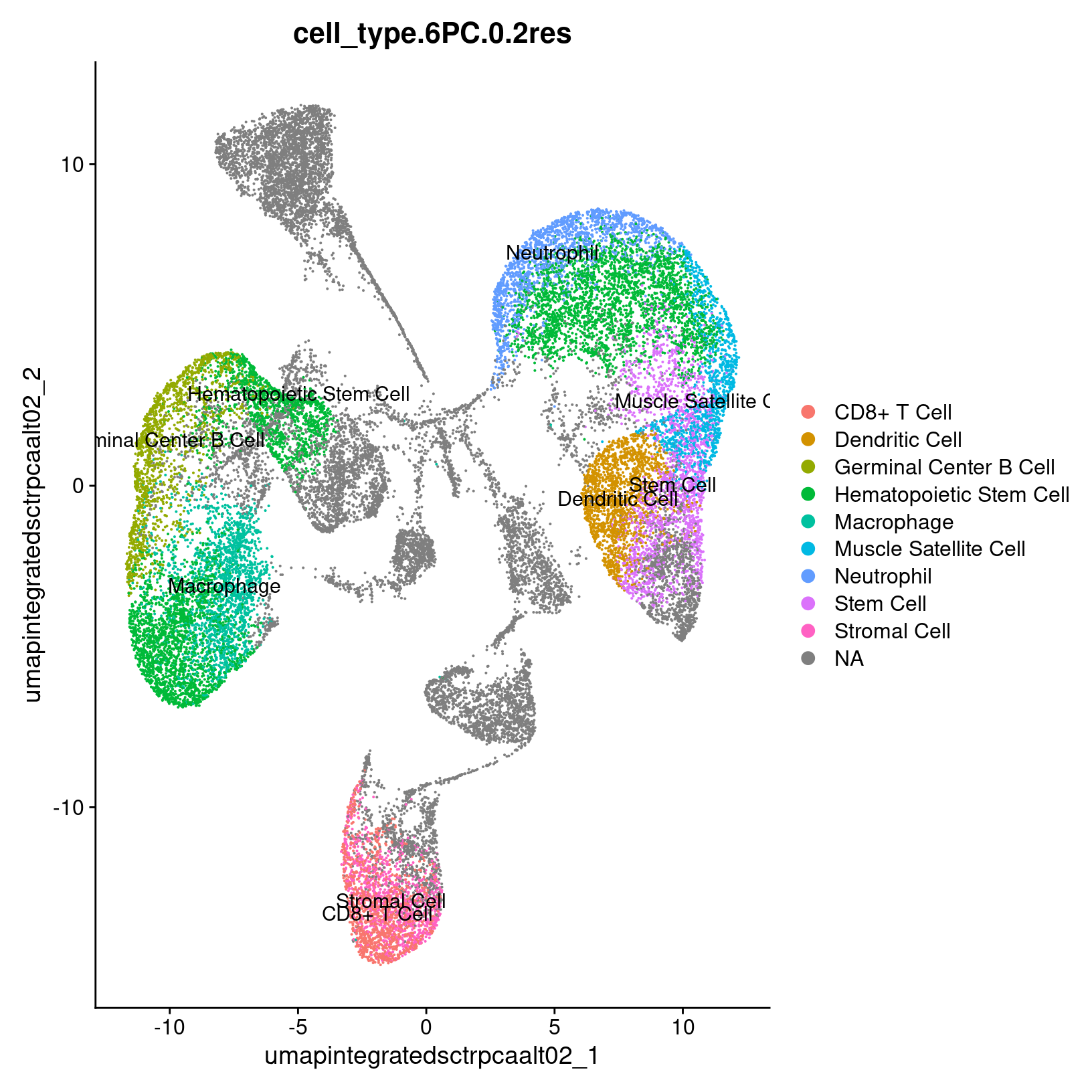

# Save the plot to file
# output to file, including the number of PCs and resolution used to generate results
ggsave(filename = paste0('results/figures/umap_int_catch-labeled_', 
                         pcs,'PC.',res,'res','.png'),
       plot = catch_umap_plot, 
       width = 8, height = 6, units = 'in')


## ----------------------------------------------------------
## Clean up session 
rm(list=names(which(unlist(eapply(.GlobalEnv, is.ggplot))))); 
rm(catch_celltypes, catch_markers, exso3_catch, exso3_markers, new_metadata, top_5); 
gc()

            used   (Mb) gc trigger   (Mb)   max used    (Mb)
Ncells   6944763  370.9   10752860  574.3   10752860   574.3
Vcells 338468682 2582.4 1229359917 9379.3 1534788602 11709.6

## (Optional) - Save copy of exso3
saveRDS(exso3, file = paste0('results/rdata/geo_so_sct_integrated_with_markers_exercise.rds'))
rm(exso3)
gc()

            used   (Mb) gc trigger   (Mb)   max used    (Mb)
Ncells   6944784  370.9   10752860  574.3   10752860   574.3
Vcells 338468716 2582.4  983487934 7503.5 1534788602 11709.6

## BEFORE PROCEEDING TO THE NEXT SECTION or closing window - POWER DOWN AND RESTART R SESSION

---