Analysis summary and next steps
UM Bioinformatics Core Workshop Team
2025-10-16
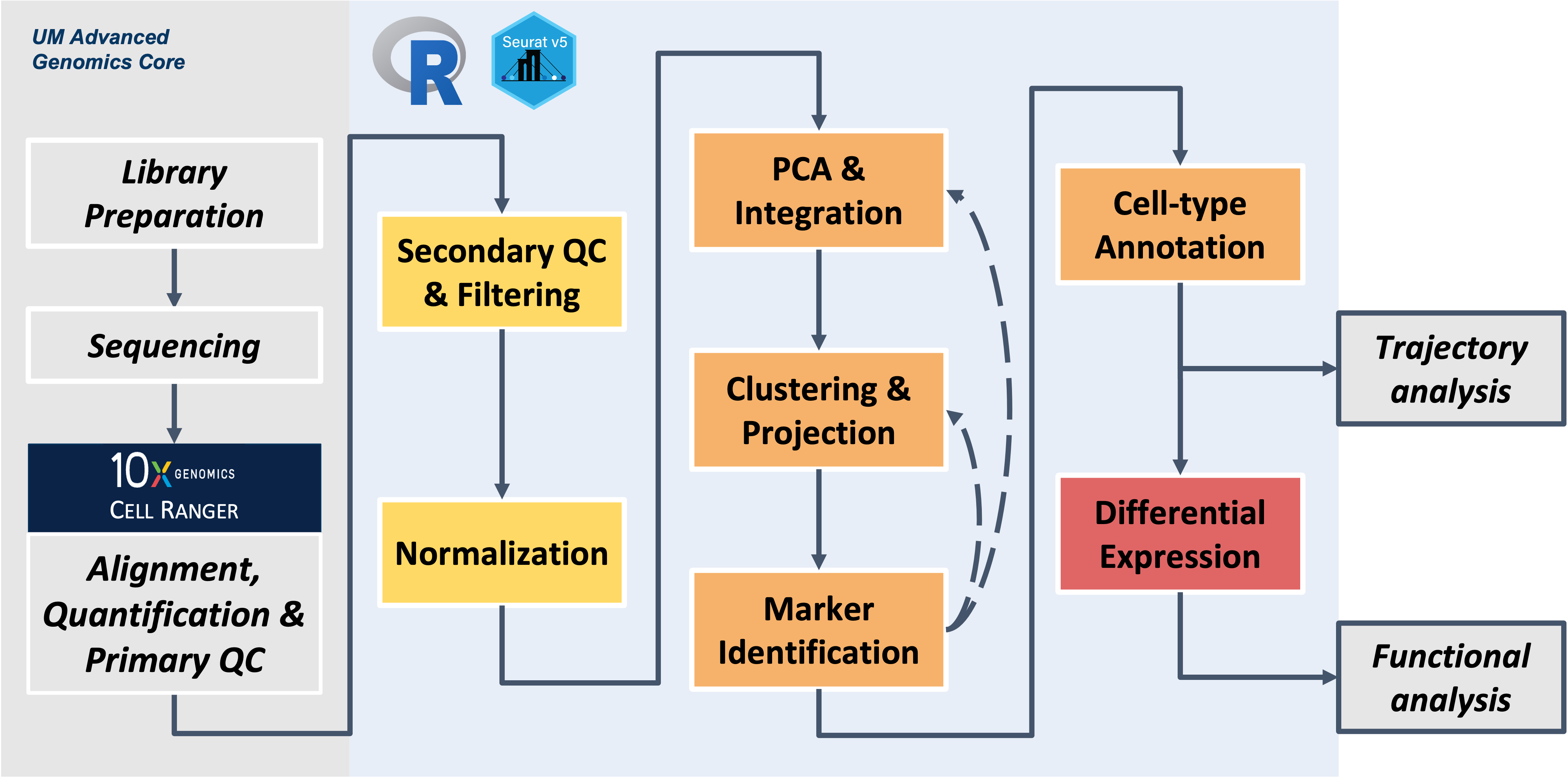
Workflow Overview
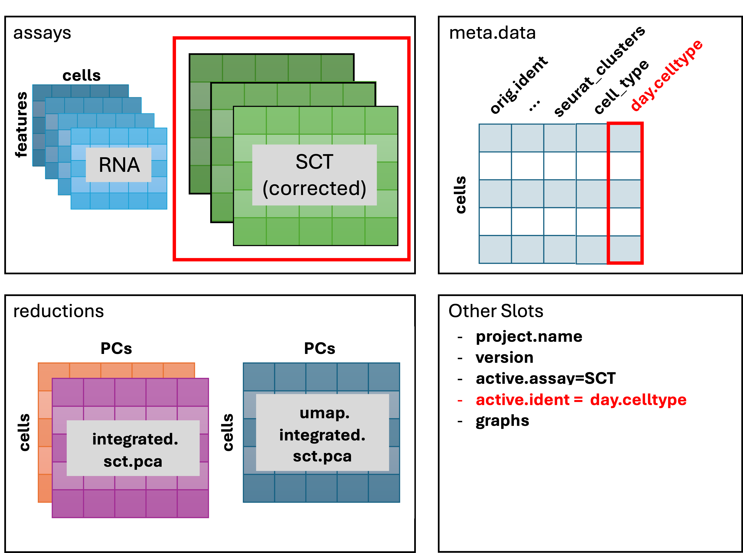
Our final Seurat object:
Key decision points in analysis and methodology
We’ve successfully analyzed our single-cell RNA-seq data,
running the following steps.
Note that the parameters we selected for the workshop are in bold. When running a different dataset, you will need to review and adjust these choices as appropriate.
| Step | Goal | Parameters/tools used in workshop |
|---|---|---|
| Loading data | Initialize Seurat object | Read10x(): you will need to specify the
paths to CellRanger directories that contain the
feature_barcode_matrix “triples” |
| Secondary QC filtering | Identify healthy, single-cells for downstream analysis | nFeature_RNA < 300 (genes per
cell), max percent.mt < 15 (%
mitochondrial genes per cell) |
| Normalization | Separate biological effects from technical effects | SCTransform with default parameters |
| Integration | Remove batch effects between individual or groups of samples | IntegrateLayers function, using
RPCAIntegration as the method |
| Clustering | Group populations of cells with similar expression programs that correspond to cell-types and/or sub-types of interest | FindNeighbors and
FindClusters using default Louvain algorithm with
10 PCs and 0.4 resolution |
| Annotation | Identify cell-types present in data | scCATCH to generate predicted cell-types
and expression plots of marker genes manually pulled from the
literature to finalize the annotations |
| Differential expression comparisons | Identify genes that are impacted by the experimental groups/condition within a given cell-type | FindMarkers with
wilcox as the statistical test used for the
standard comparisons and DESeq used for the
psuedobulk comparisons |
Organizing the tools and parameters used in our analysis can also be helpful for creating a more descriptive methods summary, like what would be included in a paper.
Example publication style methods
Data analysis
University of Michigan Biomedical Research Core Facilities Advanced Genomics Core executed 10x Genomics Cell Ranger (v9.0.0) to perform sample de-multiplexing, barcode processing, and single cell gene counting (Alignment, Barcoding and UMI Count); alignments were against mm10-2020-A and included intronic sequence. The Cell Ranger filtered barcode feature matrix was used as input to downstream analysis.
All analysis and graphics were generated in R (v4.4.1) [1]. Analysis was performed primarily using the Seurat package (v5.0.1) [2]. Cells with extreme values (which indicate low complexity, doublets, or apoptotic cells) were excluded by filtering to include only cells where Genes/cell >300 and % mitochondrial < 15% resulting in approximately 600-5,600 cells per sample after filtering. Counts were then normalized using the SCTransform method with default parameters [3].
Normalized data were integrated using the RPCA method (IntegrateLayers function with “SCT” as normalization method. Principal Component Analysis (PCA) was then performed and the first 10 significant components were used for finding nearest neighbors followed by graph-based, semi-unsupervised Louvain clustering into distinct populations (resolution = 0.4). All uniform manifold approximation and projection (UMAP) plots were generated using default settings [4]. To identify marker genes, the clusters in the integrated data were compared pairwise for differential gene expression using Wilcoxon rank-sum test for single-cell gene expression (FindAllMarkers function; default parameters) [5]. Additional marker genes and cell-type predictions were generated with scCATCH (3.2.2) [6].
To identify differentially expressed (DE) genes within the total population, Case and Control samples were compared pairwise for differential expression expression (FindAllMarkers function; log2FC = 1.5; test.use = “Wilcoxon”). For each cluster, the results were further limited to significantly different genes (Benjamini-Hochberg adjusted p-value <= 0.05). Intra-cluster case-vs-control pseudo bulk comparisons were analyzed using DESeq2 (v1.44.0) [7].
References
- R Core Team (2019). R: A language and environment for statistical computing. R Foundation for Statistical Computing, Vienna, Austria. https://www.R-project.org/.
- Stuart T, Butler A, Hoffman P, Hafemeister C, Papalexi E, III WMM, Stoeckius M, Smibert P, Satija R (2018). “Comprehensive integration of single cell data.” bioRxiv. doi: 10.1101/460147, https://www.biorxiv.org/content/10.1101/460147v1
- Hafemeister, C., Satija, R (2019). Normalization and variance stabilization of single-cell RNA-seq data using regularized negative binomial regression. Genome Biol 20, 296. https://doi.org/10.1186/s13059-019-1874-1
- Becht, E. et al (2018). Dimensionality reduction for visualizing single-cell data using UMAP. Nat. Biotechnol. 37, 38–44 .
- Myles Hollander and Douglas A. Wolfe (1973). Nonparametric Statistical Methods. New York: John Wiley & Sons. Pages 68–75.
- Shao et al (2020), scCATCH:Automatic Annotation on Cell Types of Clusters from Single-Cell RNA Sequencing Data, iScience, Volume 23, Issue 3. doi: 10.1016/j.isci.2020.100882.
- Love MI, Huber W, Anders S (2014). “Moderated estimation of fold change and dispersion for RNA-seq data with DESeq2.” Genome Biology, 15, 550. doi:10.1186/s13059-014-0550-8.
Methods from original paper
The example dataset used in the workshop was inspired by Sorkin et al. so it can also be helpful to consider the methods section from the original paper.
Sorkin et al. Methods
the experimental methods below were excerpted directly from:
- Sorkin, Michael et al. “Regulation of heterotopic
ossification by monocytes in a mouse model of aberrant wound
healing.” Nature communications vol. 11,1 722. 5
Feb. 2020.
https://pubmed.ncbi.nlm.nih.gov/32024825/
Tissues harvested from the extremity injury site were digested for 45 min in 0.3% Type 1 Collagenase and 0.4% Dispase II (Gibco) in Roswell Park Memorial Institute (RPMI) medium at 37 °C under constant agitation at 120 rpm. Digestions were subsequently quenched with 10% FBS RPMI and filtered through 40μm sterile strainers. Cells were then washed in PBS with 0.04% BSA, counted and resuspended at a concentration of ~1000 cells/μl. Cell viability was assessed with Trypan blue exclusion on a Countess II (Thermo Fisher Scientific) automated counter and only samples with >85% viability were processed for further sequencing.
University of Michigan Biomedical Research Core Facilities Advanced Genomics Core generated single-cell 3’ libraries on the 10× Genomics Chromium Controller following the manufacturers protocol for the v2 reagent kit (10× Genomics, Pleasanton, CA, USA). Cell suspensions were loaded onto a Chromium Single-Cell A chip along with reverse transcription (RT) master mix and single cell 3’ gel beads, aiming for 2000–6000 cells per channel. In this experiment, 8700 cells were encapsulated into emulsion droplets at a concentration of 700–1200 cells/ul which targets 5000 single cells with an expected multiplet rate of 3.9%. Following generation of single-cell gel bead-in-emulsions (GEMs), reverse transcription was performed and the resulting Post GEM-RT product was cleaned up using DynaBeads MyOne Silane beads (Thermo Fisher Scientific, Waltham, MA, USA). The cDNA was amplified, SPRIselect (Beckman Coulter, Brea, CA, USA) cleaned and quantified then enzymatically fragmented and size selected using SPRIselect beads to optimize the cDNA amplicon size prior to library construction. An additional round of double-sided SPRI bead cleanup is performed after end repair and A-tailing. Another single-sided cleanup is done after adapter ligation. Indexes were added during PCR amplification and a final double-sided SPRI cleanup was performed. Libraries were quantified by Kapa qPCR for Illumina Adapters (Roche) and size was determined by Agilent tapestation D1000 tapes. Read 1 primer sequence are added to the molecules during GEM incubation. P5, P7 and sample index and read 2 primer sequence are added during library construction via end repair, A-tailing, adaptor ligation and PCR. Libraries were generated with unique sample indices (SI) for each sample. Libraries were sequenced on a HiSeq 4000, (Illumina, San Diego, CA, USA) using a HiSeq 4000 PE Cluster Kit (PN PE-410-1001) with HiSeq 4000 SBS Kit (100 cycles, PN FC-410-1002) reagents, loaded at 200 pM following Illumina’s denaturing and dilution recommendations. The run configuration was 26 × 8 × 98 cycles for Read 1, Index and Read 2, respectively.
Session Info
Additionally, the sessioninfo::session_info function (or
its predecessor base function sessionInfo) produces a list
of the relevant versions of R and all the libraries that were loaded in
the analysis. While this level of detail is usually most useful for
troubleshooting, it’s helpful to preserve this information for your
records and to include the output when asking for help, particularly in
public forums.
Session Info
This info is generally not included in main body of a paper, but you
will get serious reproducibility street-cred if it shows up in
supplemental. 😎
################################################################################
# Print out details about this R install, session, and loaded libraries
#
# You can use the built-in command sessionInfo(); we prefer
# sessioninfo::session_info() for the nicer formatting.
# Note, you may have to install the sessioninfo package:
# install.packages('sessioninfo');

sessioninfo::session_info()
─ Session info ───────────────────────────────────────────────────────────────────────────────────────────────────────────────────────────────────────────────────────────────────────
setting value
version R version 4.5.0 (2025-04-11)
os Ubuntu 22.04.5 LTS
system x86_64, linux-gnu
ui RStudio
language (EN)
collate C.UTF-8
ctype C.UTF-8
tz America/Detroit
date 2025-10-16
rstudio 2024.12.1+563 Kousa Dogwood (server)
pandoc 3.2 @ /usr/lib/rstudio-server/bin/quarto/bin/tools/x86_64/ (via rmarkdown)
quarto 1.5.57 @ /usr/lib/rstudio-server/bin/quarto/bin/quarto
─ Packages ───────────────────────────────────────────────────────────────────────────────────────────────────────────────────────────────────────────────────────────────────────────
package * version date (UTC) lib source
abind 1.4-8 2024-09-12 [2] CRAN (R 4.5.0)
assertthat 0.2.1 2019-03-21 [2] CRAN (R 4.5.0)
Biobase 2.68.0 2025-04-15 [2] Bioconductor 3.21 (R 4.5.0)
BiocGenerics 0.54.0 2025-04-15 [2] Bioconductor 3.21 (R 4.5.0)
BiocParallel 1.42.1 2025-06-01 [2] Bioconductor 3.21 (R 4.5.0)
bit 4.6.0 2025-03-06 [2] CRAN (R 4.5.0)
bit64 4.6.0-1 2025-01-16 [2] CRAN (R 4.5.0)
BPCells * 0.2.0 2024-07-18 [2] Github (bnprks/BPCells@5677cf1)
bslib 0.9.0 2025-01-30 [2] CRAN (R 4.5.0)
cachem 1.1.0 2024-05-16 [2] CRAN (R 4.5.0)
cli 3.6.5 2025-04-23 [2] CRAN (R 4.5.0)
cluster 2.1.8.1 2025-03-12 [2] CRAN (R 4.5.0)
codetools 0.2-20 2024-03-31 [2] CRAN (R 4.5.0)
cowplot 1.2.0 2025-07-07 [2] CRAN (R 4.5.0)
crayon 1.5.3 2024-06-20 [2] CRAN (R 4.5.0)
data.table 1.17.8 2025-07-10 [2] CRAN (R 4.5.0)
DelayedArray 0.34.1 2025-04-17 [2] Bioconductor 3.21 (R 4.5.0)
deldir 2.0-4 2024-02-28 [2] CRAN (R 4.5.0)
DESeq2 1.48.1 2025-05-11 [2] Bioconductor 3.21 (R 4.5.0)
digest 0.6.37 2024-08-19 [2] CRAN (R 4.5.0)
dotCall64 1.2 2024-10-04 [2] CRAN (R 4.5.0)
dplyr * 1.1.4 2023-11-17 [2] CRAN (R 4.5.0)
evaluate 1.0.4 2025-06-18 [2] CRAN (R 4.5.0)
farver 2.1.2 2024-05-13 [2] CRAN (R 4.5.0)
fastDummies 1.7.5 2025-01-20 [2] CRAN (R 4.5.0)
fastmap 1.2.0 2024-05-15 [2] CRAN (R 4.5.0)
fitdistrplus 1.2-4 2025-07-03 [2] CRAN (R 4.5.0)
forcats * 1.0.0 2023-01-29 [2] CRAN (R 4.5.0)
future 1.58.0 2025-06-05 [2] CRAN (R 4.5.0)
future.apply 1.20.0 2025-06-06 [2] CRAN (R 4.5.0)
generics 0.1.4 2025-05-09 [2] CRAN (R 4.5.0)
GenomeInfoDb 1.44.0 2025-04-15 [2] Bioconductor 3.21 (R 4.5.0)
GenomeInfoDbData 1.2.14 2025-06-12 [2] Bioconductor
GenomicRanges 1.60.0 2025-04-15 [2] Bioconductor 3.21 (R 4.5.0)
ggplot2 * 3.5.2 2025-04-09 [2] CRAN (R 4.5.0)
ggrepel 0.9.6 2024-09-07 [2] CRAN (R 4.5.0)
ggridges 0.5.6 2024-01-23 [2] CRAN (R 4.5.0)
globals 0.18.0 2025-05-08 [2] CRAN (R 4.5.0)
glue 1.8.0 2024-09-30 [2] CRAN (R 4.5.0)
goftest 1.2-3 2021-10-07 [2] CRAN (R 4.5.0)
gridExtra 2.3 2017-09-09 [2] CRAN (R 4.5.0)
gtable 0.3.6 2024-10-25 [2] CRAN (R 4.5.0)
hms 1.1.3 2023-03-21 [2] CRAN (R 4.5.0)
htmltools 0.5.8.1 2024-04-04 [2] CRAN (R 4.5.0)
htmlwidgets 1.6.4 2023-12-06 [2] CRAN (R 4.5.0)
httpuv 1.6.16 2025-04-16 [2] CRAN (R 4.5.0)
httr 1.4.7 2023-08-15 [2] CRAN (R 4.5.0)
ica 1.0-3 2022-07-08 [2] CRAN (R 4.5.0)
igraph 2.1.4 2025-01-23 [2] CRAN (R 4.5.0)
IRanges 2.42.0 2025-04-15 [2] Bioconductor 3.21 (R 4.5.0)
irlba 2.3.5.1 2022-10-03 [2] CRAN (R 4.5.0)
jquerylib 0.1.4 2021-04-26 [2] CRAN (R 4.5.0)
jsonlite 2.0.0 2025-03-27 [2] CRAN (R 4.5.0)
kableExtra * 1.4.0.15 2025-06-12 [4] Github (haozhu233/kableExtra@2f58f89)
KernSmooth 2.23-26 2025-01-01 [2] CRAN (R 4.5.0)
klippy * 0.0.0.9500 2025-06-12 [4] Github (umich-brcf-bioinf/workshop-klippy@a1be090)
knitr * 1.50 2025-03-16 [2] CRAN (R 4.5.0)
labeling 0.4.3 2023-08-29 [2] CRAN (R 4.5.0)
later 1.4.2 2025-04-08 [2] CRAN (R 4.5.0)
lattice 0.22-7 2025-04-02 [2] CRAN (R 4.5.0)
lazyeval 0.2.2 2019-03-15 [2] CRAN (R 4.5.0)
leiden 0.4.3.1 2023-11-17 [2] CRAN (R 4.5.0)
lifecycle 1.0.4 2023-11-07 [2] CRAN (R 4.5.0)
limma 3.64.1 2025-05-25 [2] Bioconductor 3.21 (R 4.5.0)
listenv 0.9.1 2024-01-29 [2] CRAN (R 4.5.0)
lmtest 0.9-40 2022-03-21 [2] CRAN (R 4.5.0)
locfit 1.5-9.12 2025-03-05 [2] CRAN (R 4.5.0)
lubridate * 1.9.4 2024-12-08 [2] CRAN (R 4.5.0)
magrittr 2.0.3 2022-03-30 [2] CRAN (R 4.5.0)
MASS 7.3-65 2025-02-28 [2] CRAN (R 4.5.0)
Matrix 1.7-3 2025-03-11 [2] CRAN (R 4.5.0)
MatrixGenerics 1.20.0 2025-04-15 [2] Bioconductor 3.21 (R 4.5.0)
matrixStats 1.5.0 2025-01-07 [2] CRAN (R 4.5.0)
mime 0.13 2025-03-17 [2] CRAN (R 4.5.0)
miniUI 0.1.2 2025-04-17 [2] CRAN (R 4.5.0)
nlme 3.1-168 2025-03-31 [2] CRAN (R 4.5.0)
parallelly 1.45.0 2025-06-02 [2] CRAN (R 4.5.0)
patchwork 1.3.1 2025-06-21 [2] CRAN (R 4.5.0)
pbapply 1.7-2 2023-06-27 [2] CRAN (R 4.5.0)
pillar 1.11.0 2025-07-04 [2] CRAN (R 4.5.0)
pkgconfig 2.0.3 2019-09-22 [2] CRAN (R 4.5.0)
plotly 4.11.0 2025-06-19 [2] CRAN (R 4.5.0)
plyr 1.8.9 2023-10-02 [2] CRAN (R 4.5.0)
png 0.1-8 2022-11-29 [2] CRAN (R 4.5.0)
polyclip 1.10-7 2024-07-23 [2] CRAN (R 4.5.0)
presto 1.0.0 2024-02-06 [2] Github (immunogenomics/presto@31dc97f)
prettyunits 1.2.0 2023-09-24 [2] CRAN (R 4.5.0)
progress 1.2.3 2023-12-06 [2] CRAN (R 4.5.0)
progressr 0.15.1 2024-11-22 [2] CRAN (R 4.5.0)
promises 1.3.3 2025-05-29 [2] CRAN (R 4.5.0)
purrr * 1.1.0 2025-07-10 [2] CRAN (R 4.5.0)
R6 2.6.1 2025-02-15 [2] CRAN (R 4.5.0)
ragg 1.4.0 2025-04-10 [2] CRAN (R 4.5.0)
RANN 2.6.2 2024-08-25 [2] CRAN (R 4.5.0)
RColorBrewer 1.1-3 2022-04-03 [2] CRAN (R 4.5.0)
Rcpp 1.1.0 2025-07-02 [2] CRAN (R 4.5.0)
RcppAnnoy 0.0.22 2024-01-23 [2] CRAN (R 4.5.0)
RcppHNSW 0.6.0 2024-02-04 [2] CRAN (R 4.5.0)
readr * 2.1.5 2024-01-10 [2] CRAN (R 4.5.0)
reshape2 1.4.4 2020-04-09 [2] CRAN (R 4.5.0)
reticulate 1.42.0 2025-03-25 [2] CRAN (R 4.5.0)
rlang 1.1.6 2025-04-11 [2] CRAN (R 4.5.0)
rmarkdown * 2.29 2024-11-04 [2] CRAN (R 4.5.0)
ROCR 1.0-11 2020-05-02 [2] CRAN (R 4.5.0)
RSpectra 0.16-2 2024-07-18 [2] CRAN (R 4.5.0)
rstudioapi 0.17.1 2024-10-22 [2] CRAN (R 4.5.0)
Rtsne 0.17 2023-12-07 [2] CRAN (R 4.5.0)
S4Arrays 1.8.1 2025-06-01 [2] Bioconductor 3.21 (R 4.5.0)
S4Vectors 0.46.0 2025-04-15 [2] Bioconductor 3.21 (R 4.5.0)
sass 0.4.10 2025-04-11 [2] CRAN (R 4.5.0)
scales 1.4.0 2025-04-24 [2] CRAN (R 4.5.0)
scattermore 1.2 2023-06-12 [2] CRAN (R 4.5.0)
scCATCH * 3.2.2 2023-04-23 [2] CRAN (R 4.5.0)
sctransform 0.4.2 2025-04-30 [2] CRAN (R 4.5.0)
sessioninfo 1.2.3 2025-02-05 [2] CRAN (R 4.5.0)
Seurat * 5.1.0 2024-05-10 [2] CRAN (R 4.5.0)
SeuratObject * 5.1.0 2025-04-22 [2] CRAN (R 4.5.0)
shiny 1.11.1 2025-07-03 [2] CRAN (R 4.5.0)
sp * 2.2-0 2025-02-01 [2] CRAN (R 4.5.0)
spam 2.11-1 2025-01-20 [2] CRAN (R 4.5.0)
SparseArray 1.8.0 2025-04-15 [2] Bioconductor 3.21 (R 4.5.0)
spatstat.data 3.1-6 2025-03-17 [2] CRAN (R 4.5.0)
spatstat.explore 3.4-3 2025-05-21 [2] CRAN (R 4.5.0)
spatstat.geom 3.4-1 2025-05-20 [2] CRAN (R 4.5.0)
spatstat.random 3.4-1 2025-05-20 [2] CRAN (R 4.5.0)
spatstat.sparse 3.1-0 2024-06-21 [2] CRAN (R 4.5.0)
spatstat.univar 3.1-3 2025-05-08 [2] CRAN (R 4.5.0)
spatstat.utils 3.1-4 2025-05-15 [2] CRAN (R 4.5.0)
statmod 1.5.0 2023-01-06 [2] CRAN (R 4.5.0)
stringi 1.8.7 2025-03-27 [2] CRAN (R 4.5.0)
stringr * 1.5.1 2023-11-14 [2] CRAN (R 4.5.0)
SummarizedExperiment 1.38.1 2025-04-30 [2] Bioconductor 3.21 (R 4.5.0)
survival 3.8-3 2024-12-17 [2] CRAN (R 4.5.0)
svglite 2.2.1 2025-05-12 [3] CRAN (R 4.5.0)
systemfonts 1.2.3 2025-04-30 [2] CRAN (R 4.5.0)
tensor 1.5.1 2025-06-17 [2] CRAN (R 4.5.0)
textshaping 1.0.1 2025-05-01 [2] CRAN (R 4.5.0)
tibble * 3.3.0 2025-06-08 [2] CRAN (R 4.5.0)
tidyr * 1.3.1 2024-01-24 [2] CRAN (R 4.5.0)
tidyselect 1.2.1 2024-03-11 [2] CRAN (R 4.5.0)
tidyverse * 2.0.0 2023-02-22 [2] CRAN (R 4.5.0)
timechange 0.3.0 2024-01-18 [2] CRAN (R 4.5.0)
tzdb 0.5.0 2025-03-15 [2] CRAN (R 4.5.0)
UCSC.utils 1.4.0 2025-04-15 [2] Bioconductor 3.21 (R 4.5.0)
utf8 1.2.6 2025-06-08 [2] CRAN (R 4.5.0)
uwot 0.2.3 2025-02-24 [2] CRAN (R 4.5.0)
vctrs 0.6.5 2023-12-01 [2] CRAN (R 4.5.0)
viridisLite 0.4.2 2023-05-02 [2] CRAN (R 4.5.0)
vroom 1.6.5 2023-12-05 [2] CRAN (R 4.5.0)
withr 3.0.2 2024-10-28 [2] CRAN (R 4.5.0)
xfun 0.52 2025-04-02 [2] CRAN (R 4.5.0)
xml2 1.3.8 2025-03-14 [2] CRAN (R 4.5.0)
xtable 1.8-4 2019-04-21 [2] CRAN (R 4.5.0)
XVector 0.48.0 2025-04-15 [2] Bioconductor 3.21 (R 4.5.0)
yaml 2.3.10 2024-07-26 [2] CRAN (R 4.5.0)
zoo 1.8-14 2025-04-10 [2] CRAN (R 4.5.0)
[1] /home/workshop/cgates/R/x86_64-pc-linux-gnu-library/4.5
[2] /efs/workshop/R/library
[3] /efs/workshop/ifun/R/library
[4] /efs/workshop/R/workshop-dev-libs
[5] /usr/local/lib/R/site-library
[6] /usr/lib/R/site-library
[7] /usr/lib/R/library
* ── Packages attached to the search path.
──────────────────────────────────────────────────────────────────────────────────────────────────────────────────────────────────────────────────────────────────────────────────────
Troubleshooting and alternative approaches
As we discussed in the workshop, single-cell analysis can be very iterative with the impact of choices made earlier in the analysis might not being apparent until later in the analysis and often we can only evaluate how well those choices reflect the biological context and/or the granularity of our biological question until the end of the analysis (ask me how I know).
To help with future troubleshooting - here’s a reiteration the key analysis steps, what we might see that would indicate a need to go back to and revise the choices made at that step, and some non-exhaustive alternative approaches or tools:
| Step | Issue & potential alternative(s) |
|---|---|
| Secondary QC filtering | If you see poor clustering (one big blob) or
clusters that seem be driven by quality metrics like total
counts or correspond to stress/debris instead of biological relevant
cell-types, then re-filtering with more stringent
thresholds might help, including adding a threshold for
nCount_RNA (total counts per cell) |
| Secondary QC filtering | If you are missing expected cell type(s) after clustering that might have a different average number of genes expressed or total counts (like blood cells or T-cells) or with a higher expected % mitochondrial genes, then re-filtering with more relaxed thresholds could help to recover those cells and allow them to be included in the downstream analysis |
| Normalization | If clusters correspond more to technical factors than biologically relevant cell-types, then covariates for those technical factors may need to added to the normalization model or a different normalization approach might be needed |
| Normalization | If there is a low total % variance explained when looking at the PCs and covariates for one or more technical factor was included in the normalization step, then the normalization step may have overcorrected and some of the biological variation that corresponds to cell-types was also removed. Check to see if any of the known technical covariates have evidence of skewing the data and limit the model to a minimal number of covariates. |
| Integration | We chose to use RPCA for our integration
but there are other integration options. If RPCA is
not sufficient to correct observed batch effects and all
samples/conditions are expected to share the same cell-types, a
CCA might be worth trying. If
neither RPCA or CCA work
well, another option might be Harmony, which uses a
different approach and parameters to correct for batch while
preserving unique cell populations.
|
| Clustering | If the clustering looks too blobby (e.g. few or no distinct clusters), then you may have over corrected by including the wrong or too many covariates in the normalization step and/or used too few PCs to define distinct celltypes. Additionally, while we used the default Louvain algorithm for cluster determination, alternative algorithms are supported including Leiden clustering. |
| Cell type annotation | While we used scCATCH, if more specific
example data and annotations are available for your tissue (e.g. brain
or blood/immune) or if the predictions from scCATCH don’t
seem relevant to your tissue and/or experimental question, there are
other sources and tools available that might be worth trying like
CellMatch_2.0 or Azimuth or a label transfer
using a similar dataset. |
| Differential expression | While we used Wilcoxin and
DESeq2 for our differential expression testing, other tools
like MAST or EdgeR can also be used and/or
more complex models with covariates could be used. |
| Differential expression | We choose a general cutoff
(p_val_adj < 0.05 &
abs(avg_log2FC) > 1.5)) to call DE genes but if
there are not enough DE genes, then it might make sense
to relax those cutoff for some clusters. |
| Differential expression | Conversely if there are too many DE genes to use for downstream steps like functional enrichments, then it might be necessary to make the cutoffs more stringent for those specific comparisons. |
| Subclustering | While we weren’t able to cover this topic, if you wanted to know what general cell-types present but are more interested in comparing the proportions or gene expression between subtypes of a more general cell population (e.g. it’s helpful to know how many B-cell, T-cells, etc are generally in your PBMC samples but you are most interested in of subtypes of effector T-cells), it might be worth considering running subclustering after initial clustering and annotation. |
Downstream approaches
Although outside the scope of the workshop, there are many other possible avenues of exploration and analysis for scRNA-seq data beyond differential expression within clusters, either with each cell as a replicate or using a pseudobulk approach. This includes but is not limited to:
Integration with other modalities (e.g. ATAC-seq, VDJ, etc.)
Subclustering clusters of interest - see HBC’s summary on subclustering, Seurat’s findSubcCluster documentation and this related issue thread
Trajectory or Pseudotime analysis - see Single Cell Best Practices: Inferring Trajectories or Broad Institute’s materials on trajectory analysis
Cell - Cell communication network inference, see review by Wilk et al (2023)
Velocity analysis (note: not compatible with the flex probe based kits), see the chapter from the single-cells best practices book for detailed theory/modeling or the 10x data vignette for velocyto for a practical example in R
We would recommend looking for studies in similar tissues or with
similar experimental questions to see what kind of approaches and tools
were used to help guide your own analysis plans.
Resources for continued learning.
- Learning bioinformatic analyses is more like a process than a task.
Resources to consider:
- A CZI NDCN curated list of resources for self-guided learning
- UM Bioinformatics Core links to training resources/workshops.
- Techniques in Bash and R
- Lesson plans from the UM Bioinformatics Core’s recent Computational Foundations Workshop.
- Lessons and workshops in Bash / Git / R / Python : Software Carpentry
- More info on NGS analysis (A decidedly
non-exhaustive list in no discernible order.)
- Lesson plans from UM Bioinformatics Core’s recent RNA-Seq Demystified Workshop. (Note this is for bulk RNA-Seq.)
- Training materials from Harvard Chan Bioinformatics Core.
- Orchestrating Single-Cell Analysis with Bioconductor.
- Welcome Sanger Instutute’s Analysis of single cell RNA-seq data.
- In addition to maintaining the Seurat analysis platform, New York Genome Center’s Satija lab publishes many excellent step-by-step tutorials on single-cell analysis, e.g. Seurat - Guided Clustering Tutorial. The Satija lab also hosts Single Cell Genomics Day, a live-streamed annual symposium on emerging techniques in single-cell analysis.
- Nayak, Richa, and Yasha Hasija. “A hitchhiker’s guide to
single-cell transcriptomics and data analysis pipelines.”
Genomics vol. 113,2 (2021): 606-619.
https://pubmed.ncbi.nlm.nih.gov/33485955/ - Luecken, Malte D, and Fabian J Theis. “Current best
practices in single-cell RNA-seq analysis: a tutorial.”
Molecular systems biology vol. 15,6 e8746. 19 Jun. 2019.
https://pubmed.ncbi.nlm.nih.gov/31217225/ - He, Jiangping et al. “Practical bioinformatics pipelines for
single-cell RNA-seq data analysis.” Biophysics reports vol. 8,3
(2022): 158-169.
https://www.ncbi.nlm.nih.gov/pmc/articles/PMC10189648/
- For more context on the experiments and data we referenced during
the workshop, see the source paper:
Sorkin, Michael et al. “Regulation of heterotopic ossification by monocytes in a mouse model of aberrant wound healing.” Nature communications vol. 11,1 722. 5 Feb. 2020.
https://pubmed.ncbi.nlm.nih.gov/32024825/
These materials have been adapted and extended from materials listed above. These are open access materials distributed under the terms of the Creative Commons Attribution license (CC BY 4.0), which permits unrestricted use, distribution, and reproduction in any medium, provided the original author and source are credited.
| Previous lesson | Top of this lesson | Workshop Wrap Up |
|---|